

Periodic splines
In our previous posts, we both discussed splines and periodic patterns, we will now discuss how to use splines to model periodic patterns. We have already seen that a $p$ order spline is continuous and its first $p-1$ derivatives are continuous. We can easily make it periodic by constraining the last $p$ coefficients, as we will see in the next few lines. In order to show this, we downloaded the average daily temperature from open-meteo.
import arviz as az
import arviz_plots as azp
import matplotlib.pyplot as plt
import numpy as np
import pandas as pd
import pymc as pm
import seaborn as sns

rng = sum(map(ord,'temperature'))

df = pd.read_csv('open-meteo-45.10N7.70E239m.csv', skiprows=3)

df.head()
| time | temperature_2m_mean (°C) | |
|---|---|---|
| 0 | 2010-01-01 | 3.5 |
| 1 | 2010-01-02 | -1.4 |
| 2 | 2010-01-03 | -0.6 |
| 3 | 2010-01-04 | -2.3 |
| 4 | 2010-01-05 | -1.3 |
We will here combine ordinary B-splines with periodic B-spline, so that we will be able to model local trends as well as the clear periodic component of the temperature.
The two functions to evaluate the spline weights are the following ones:
def bspline(t: np.array, x:np.array, i:int, p:int) -> float:
    """
    Returns a B-spline, defined as https://en.wikipedia.org/wiki/B-spline.

    Parameters:
    -----------
    t: np.array
    x: np.array
    i: int
    p: int

    Returns:
    np.array

    Raises:
    ------
    ValueError
       if i is not an integer between 0 and len(x)-p-1 (both included)
    """
    if i>=0 and i<len(x)-p-1:
        if p==0:
            return np.heaviside(t-x[i], 1)*np.heaviside(x[i+1]-t, 0)
        else:
            fac0 = (t-x[i])/(x[i+p]-x[i])
            fac1 = (x[i+p+1]-t)/(x[i+p+1]-x[i+1])
            return (fac0*bspline(t, x, i, p-1)+fac1*bspline(t, x, i+1, p-1))
    else:
        raise ValueError(f'Got i={i}, i must be an integer between 0 and len(x)-p-1={len(x)-p-1}')

def cyclic_bspline(t: np.array, knots: np.array, i: int, p: int) -> float:
    """
    Periodic (cyclic) B-spline basis function.

    Parameters
    ----------
    t : float or np.array
        Parameter value(s) where the basis is evaluated.
    knots : np.array
        Uniform knot vector (must be periodic-compatible).
    i : int
        Basis function index.
    p : int
        Degree.

    Returns
    -------
    float or np.array
    """
    n = len(knots) - p - 1   # number of B-spline basis functions

    # Wrap index cyclically
    i_mod = i % n

    # Base case
    if p == 0:
        return np.heaviside(t - knots[i_mod], 1) * np.heaviside(knots[i_mod + 1] - t, 0)

    # Recurrence (Cox–de Boor) with wrapped indices
    denom0 = knots[i_mod + p] - knots[i_mod]
    denom1 = knots[i_mod + p + 1] - knots[i_mod + 1]

    term0 = 0.0
    term1 = 0.0

    if denom0 != 0:
        term0 = (t - knots[i_mod]) / denom0 * cyclic_bspline(t, knots, i_mod, p - 1)

    if denom1 != 0:
        term1 = (knots[i_mod + p + 1] - t) / denom1 * cyclic_bspline(t, knots, i_mod + 1, p - 1)

    return term0 + term1
We will use order-2 splines
p_fit = 2
We can now start with the preprocessing
df['time'] = pd.to_datetime(df['time'])

df['day'] = df['time'].dt.dayofyear  # for the periodic part

df = df[['time', 'day', 'temperature_2m_mean (°C)']]

fig, ax = plt.subplots(figsize=(12, 6))
ax.scatter(df['time'], df['temperature_2m_mean (°C)'],  marker='x')
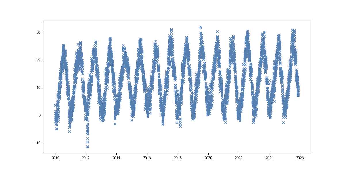
As expected, we can see a strong periodic component, as well as some local trend behavior. Since the spline is always zero at the boundaries, we will both include an constant and a trend component.
Let us now implement the splines. First of all, we will implement the periodic component.
Xday = np.minimum(df['day'], [365]*len(df))/365  # for leap years

knots_day = np.linspace(0, 1, 15)

splines_dim_day = len(knots_day)-p_fit-1

basis_day = np.array([cyclic_bspline(Xday, knots_day, i, 2) for i in range(splines_dim_day)])
We can now implement the non-periodic ones
Xdate = np.arange(len(df))/len(df)

knots_date = np.linspace(0, 1, 40)

splines_dim_date = len(knots_date)-p_fit-1

basis_date = np.array([bspline(Xdate, knots_date, i, 2) for i in range(splines_dim_date)])

# the last p basis vectors are equal to the first p ones
# in order to ensure smoothness at the boundaries

basis_day_full = np.concatenate([basis_day,  basis_day[:p_fit+1]])
We can now build and fit the model
kwargs = dict(draws=2000, tune=2000, nuts_sampler='nutpie', target_accept=0.9, random_seed=rng)

coords = {'obs': df.index, 'basis_day': range(np.shape(basis_day)[0]), 'basis_date': range(np.shape(basis_date)[0])}

with pm.Model(coords=coords) as model:
    eps = pm.Exponential('eps', 1)
    alpha = pm.Normal('alpha', mu=0, sigma=100)
    beta = pm.Normal('beta', mu=0, sigma=50, dims=('basis_day'))
    beta_full = pm.Deterministic('beta_full', pm.math.concatenate([beta, beta[:p_fit+1]]))
    gamma = pm.Normal('gamma', mu=0, sigma=50, dims=('basis_date'))
    delta = pm.Normal('delta', mu=0, sigma=50)
    mu = pm.Deterministic('mu', alpha + pm.math.dot(beta_full, basis_day_full) + pm.math.dot(gamma, basis_date) + delta*Xday)
    sigma = pm.HalfNormal('sigma', sigma=50)
    y = pm.Normal('y', mu=mu, sigma=sigma, observed=df['temperature_2m_mean (°C)'], dims=('obs'))

with model:
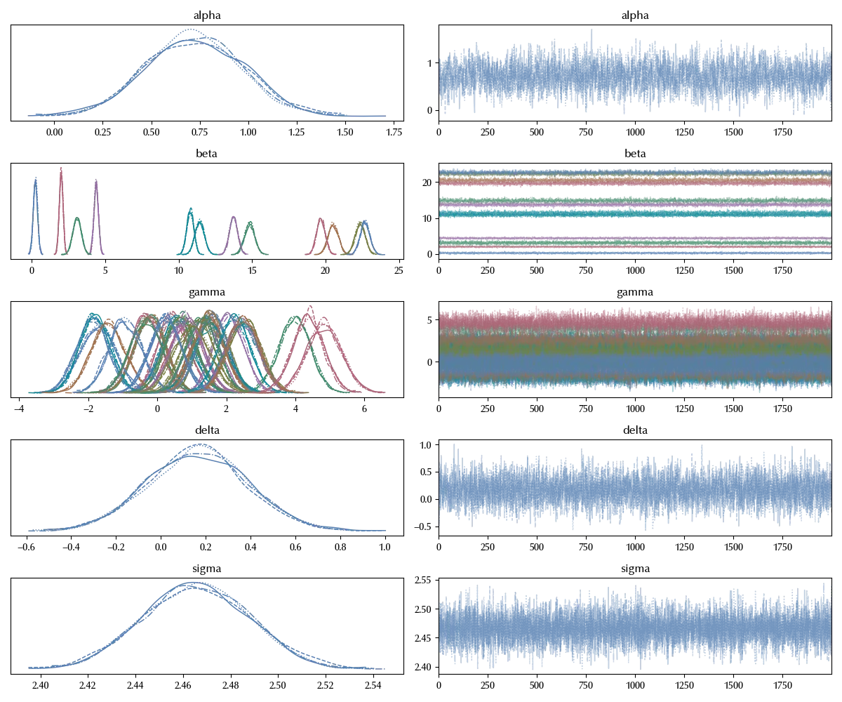
    idata = pm.sample(**kwargs)

fig, ax = plt.subplots(figsize=(15, 6))
az.plot_hdi(x=df['time'], y=idata.posterior['mu'], ax=ax, smooth=False)
fig.tight_layout()
fig, ax = plt.subplots(figsize=(15, 6))
az.plot_hdi(x=df['time'], y=idata.posterior['mu'], ax=ax, smooth=False)
sns.scatterplot(df, x='time', y='temperature_2m_mean (°C)', color='lightgray', alpha=0.4, ax=ax, marker='x')
fig.tight_layout()
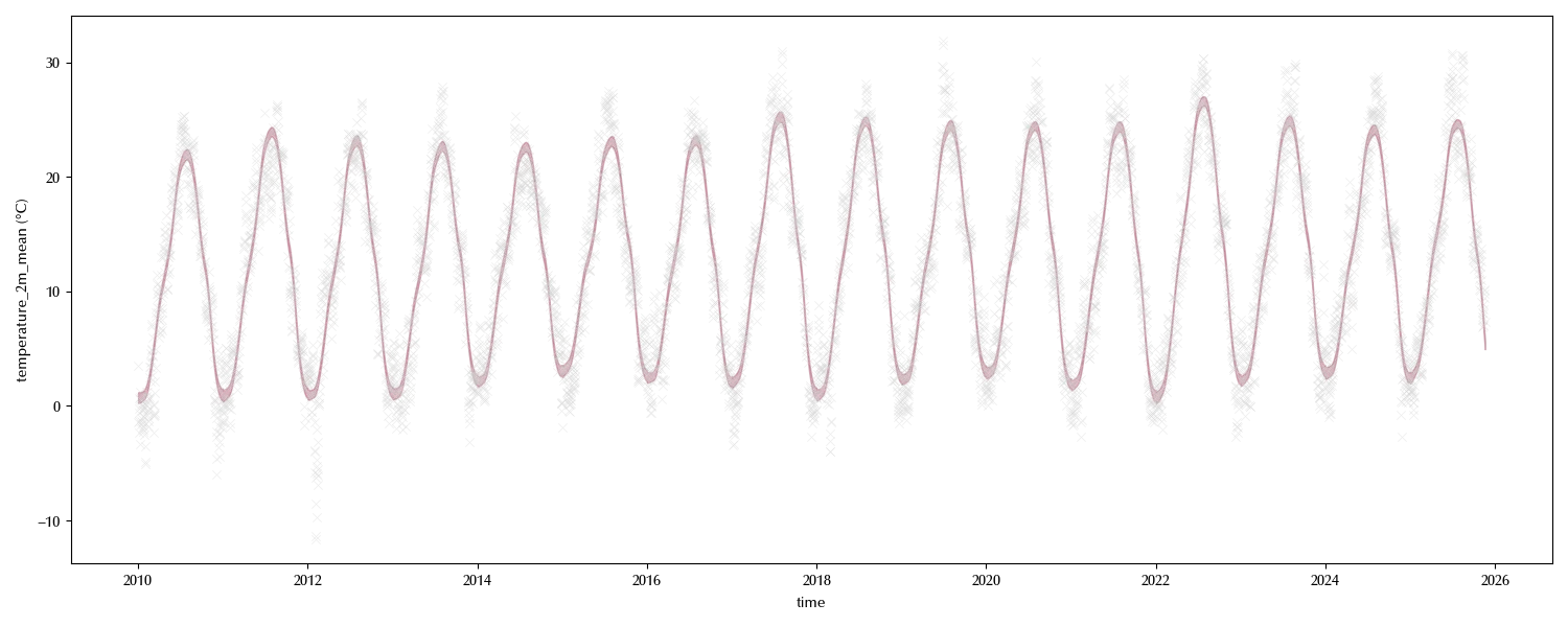
The predicted pattern clearly reproduces the observed one.
Conclusions
Spline can be adapted to account for periodic data, and in this way they are a powerful alternative to periodic GP, if you know the period of your periodic component.
%load_ext watermark

%watermark -n -u -v -iv -w -p xarray,numpyro,jax,jaxlib,pytensor
Python implementation: CPython
Python version : 3.13.9
IPython version : 9.7.0
xarray : 2025.1.2
numpyro : 0.19.0
jax : 0.8.0
jaxlib : 0.8.0
pytensor: 2.35.1
arviz_plots: 0.6.0
matplotlib : 3.10.7
pandas : 2.3.3
arviz : 0.23.0.dev0
seaborn : 0.13.2
numpy : 2.3.4
pymc : 5.26.1
Watermark: 2.5.0