Directional statistics

If you are familiar with this blog, you already know that we strongly believe that a model should encode all the relevant features of the data.

A special kind of variable we haven’t discussed up to now is the family of angular variables, that is variables which are defined on non-planar topologies.

This kind of variable is very common in contexts like movement analysis or spatial analysis, so we will dedicate them a post.

As usual, we only want to give an overview to the topic, and the interested reader will find some literature at the end of the post.

Wind direction analysis

Let us consider the dataset provided in this website where a large set of variables is provided to analyze the wind speed in a meteorological station at the Maldives.

import pandas as pd
import numpy as np
import seaborn as sns
from matplotlib import pyplot as plt
import pymc as pm
import arviz as az

df = pd.read_csv('wind-measurements_maldives_hoarafushi_wb-esmap-qc.csv')

len(df)

103884

df[['time', 'a11_wind_speed_mean', 'd11_wind_direction_mean']].head()

	time	a11_wind_speed_mean	d11_wind_direction_mean
0	10/04/2017 14:00	9999	9999
1	10/04/2017 14:10	3.174	285.696
2	10/04/2017 14:20	2.621	296.953
3	10/04/2017 14:30	2.697	288.454
4	10/04/2017 14:40	9999	9999

Let us first of all clean a little bit the dataset

df_red = df[df['a11_wind_speed_mean']<9990].copy()
df_red['time'] = pd.to_datetime(df_red['time'], format='%d/%m/%Y %H:%M')
df_red['direction'] = df_red['d11_wind_direction_mean']/360*(2.0*np.pi)

The dataset has a time frequency of 10 minutes, which is way too much for our purposes. We therefore want to average over the day, and the first obvious choice would be to take the arithmetic mean. This is however not the best choice, since is this way we wouldn’t take the circular topology into account. A proper statistics should in fact remain unchanged by replacing each angle with the same angle plus $2 \pi$, and the arithmetic mean does not have this property. A better approach is to switch to cartesian coordinates, average over the single components and only then re-compute the angle. An alternative approach could be to use the circular mean, which is the same approach just described performed assuming that the wind absolute value of the speed is always one.

df_red['cos'] = df['a11_wind_speed_mean']*np.cos(df_red['direction'])
df_red['sin'] = df['a11_wind_speed_mean']*np.sin(df_red['direction'])

df_red['Date'] = pd.to_datetime(df_red['time']) - pd.to_timedelta(7, unit='d')
df_g = df_red.groupby(pd.Grouper(key='Date', freq='W-MON'))[['cos', 'sin']].mean().reset_index().sort_values('Date')
df_g['phi'] = np.arctan2(df_g['sin'], df_g['cos'])

We can now visualize the result as follows

fig, ax = plt.subplots(subplot_kw=dict(projection='polar'))
sns.histplot(df_g, x='phi', ax=ax)
ax.set_ylabel('')
ax.set_xlabel('')
fig.tight_layout()

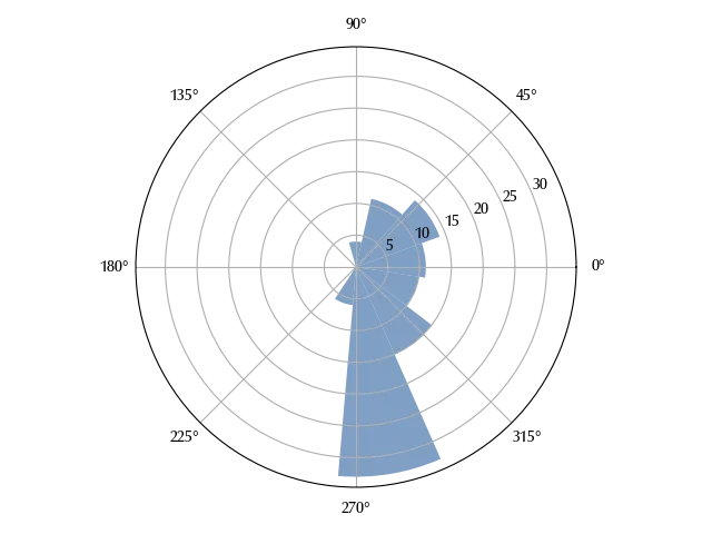
We can now try and build our model, and we must account for the non-trivial topology of our data here as we just did for the mean. A common choice in this case is the Von Mises distribution, which continuous and periodic over the entire circle.

with pm.Model() as model:
    mu = pm.Normal('mu', mu=0, sigma=10)
    kappa = pm.HalfNormal('kappa', sigma=10)
    y = pm.VonMises('y', mu=mu, kappa=kappa, observed=df_g['phi'])

rng = np.random.default_rng(42)

kwargs = dict(chains=4,
             draws=1500,
             tune=1500,
              target_accept=0.95,
             random_seed=rng,
             nuts_sampler='numpyro')

with model:
    idata = pm.sample(**kwargs)
   
az.plot_trace(idata)
fig = plt.gcf()
fig.tight_layout()

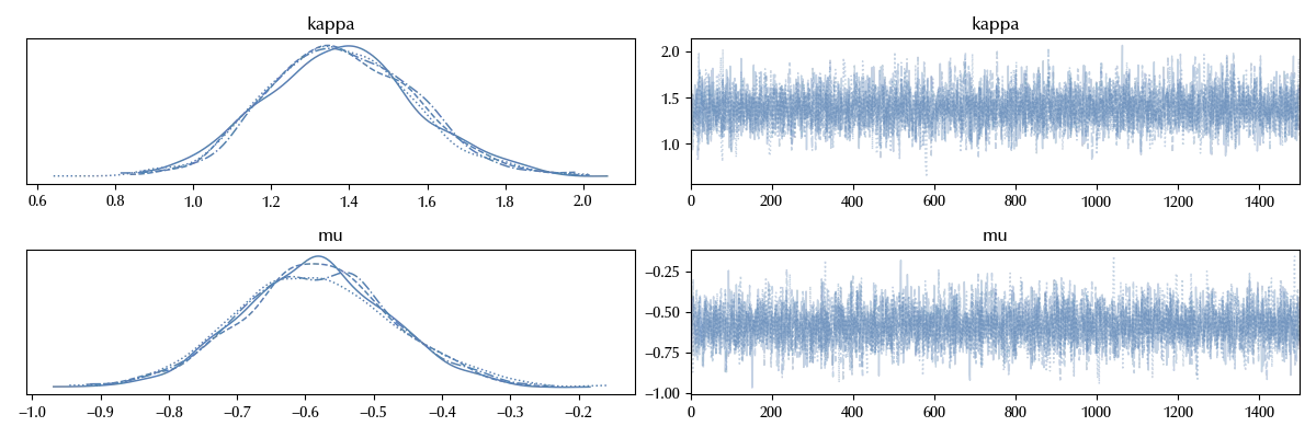
The trace looks good, let us now inspect the posterior predictive

with model:
    idata.extend(pm.sample_posterior_predictive(idata))

fig, ax = plt.subplots(subplot_kw=dict(projection='polar'))
az.plot_ppc(idata, num_pp_samples=200, ax=ax)

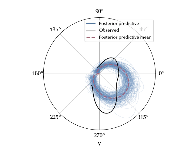
Our dataset is not appropriately described by a simple Von Mises model, and this can be easily understood by the multi modality of the data. It is in fact well known that the oceanic winds have a strong seasonal component, and this can be seen by the fact that the above histogram has a strong south component as well as a broader north-east one.

We don’t want to fix a priori the number of components, so we will use a DP mixture model. Von-Mises mixture has however an identifiability issue, since they are periodic over the circle. We will try and circumvent this issue by imposing that the variance is strictly growing with the component index.

K = 10
with pm.Model(coords={"component": np.arange(K), "obs_id": np.arange(len(df_by_day))}) as model_dp:
    alpha_c = pm.Gamma("alpha_c", 0.1, 1)
    w_c = pm.StickBreakingWeights('w_c', alpha=alpha_c, K=K-1)
    lam_c = pm.Gamma("lam_c", 0.2, 0.2, shape=(K))
    mu_c = pm.TruncatedNormal("mu_c", mu=0, sigma=np.pi, shape=(K), lower=-np.pi, upper=np.pi)
    z_c = pm.Deterministic('z_c', pm.math.cumsum(lam_c))
    y_c = pm.Mixture(
        "y_c", w_c, pm.VonMises.dist(mu=mu_c, kappa=z_c), observed=df_g['phi'])

with model_dp:
    idata_dp = pm.sample(**kwargs)

az.plot_trace(idata_dp, var_names=['alpha_c', 'mu_c', 'lam_c'])
fig = plt.gcf()
fig.tight_layout()

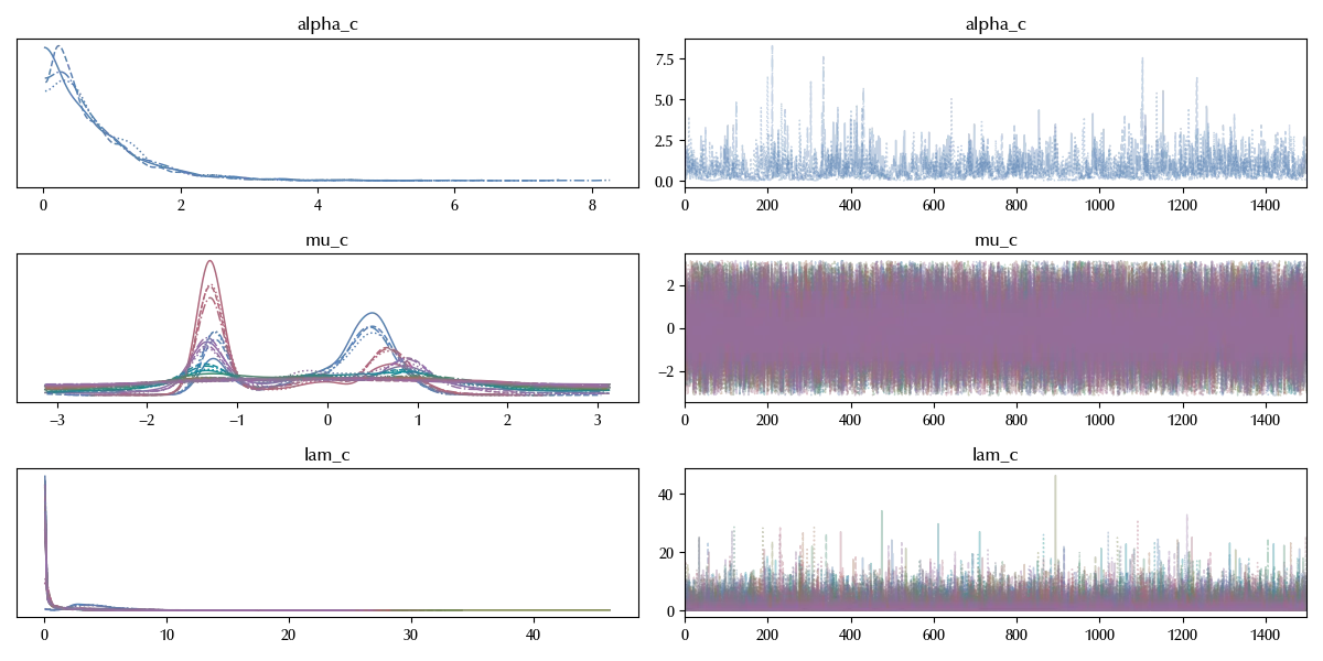
We still have some issue, but this is not a great problem for us. Let us now inspect the posterior predictive.

with model_dp:
    idata_dp.extend(pm.sample_posterior_predictive(idata_dp))

fig, ax = plt.subplots(subplot_kw=dict(projection='polar'))
az.plot_ppc(idata_dp, num_pp_samples=400, ax=ax)

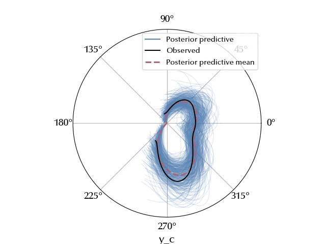
The improvement in the description of the data is clear, and again a simple model constructed by only encoding some relevant domain knowledge has shown appropriate in the description of the data.

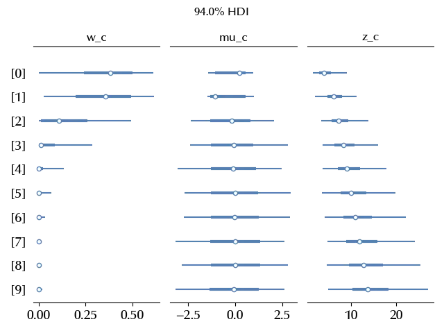
Let us finally inspect the parameters

fig, ax = plt.subplots(ncols=3, sharey=True)
az.plot_forest(idata_dp, var_names=['w_c'], combined=True, ax=ax[0])
az.plot_forest(idata_dp, var_names=['mu_c'], combined=True, ax=ax[1])
az.plot_forest(idata_dp, var_names=['z_c'], combined=True, ax=ax[2])
ax[0].set_title('w_c')
ax[1].set_title('mu_c')
ax[2].set_title('z_c')
ax[0].set_yticklabels([f"[{elem}]" for elem in range(10)][::-1])
fig.suptitle(r'94.0% HDI')
fig.tight_layout()

GP regression

We can also easily perform regression on directional data. We already know (or, at least, believe) that our data has a yearly periodic behavior, and we can encode this feature in the regression model.

df_g['X'] = (df_g['Date']-df_g['Date'].min()).dt.days/365

with pm.Model() as model_gp:
    X = pm.Data('X', df_g['X'].values.reshape((-1, 1)))
    # mu = pm.Normal('mu', mu=0, sigma=10)
    scale = pm.HalfNormal("scale", 1)
    cov_func = pm.gp.cov.Periodic(1, period=1, ls=0.1)

    # Specify the approximation with 25 basis vectors
    gp = pm.gp.HSGPPeriodic(m=25, scale=scale, cov_func=cov_func)

    # Place a GP prior over the function f.
    mu = gp.prior("mu", X=X)
    kappa = pm.HalfNormal('kappa', sigma=10)
    y = pm.VonMises('y', mu=mu, kappa=kappa, observed=df_g['phi'])

with model_gp:
    idata_gp = pm.sample(**kwargs)
    
az.plot_trace(idata_gp)
fig = plt.gcf()
fig.tight_layout()

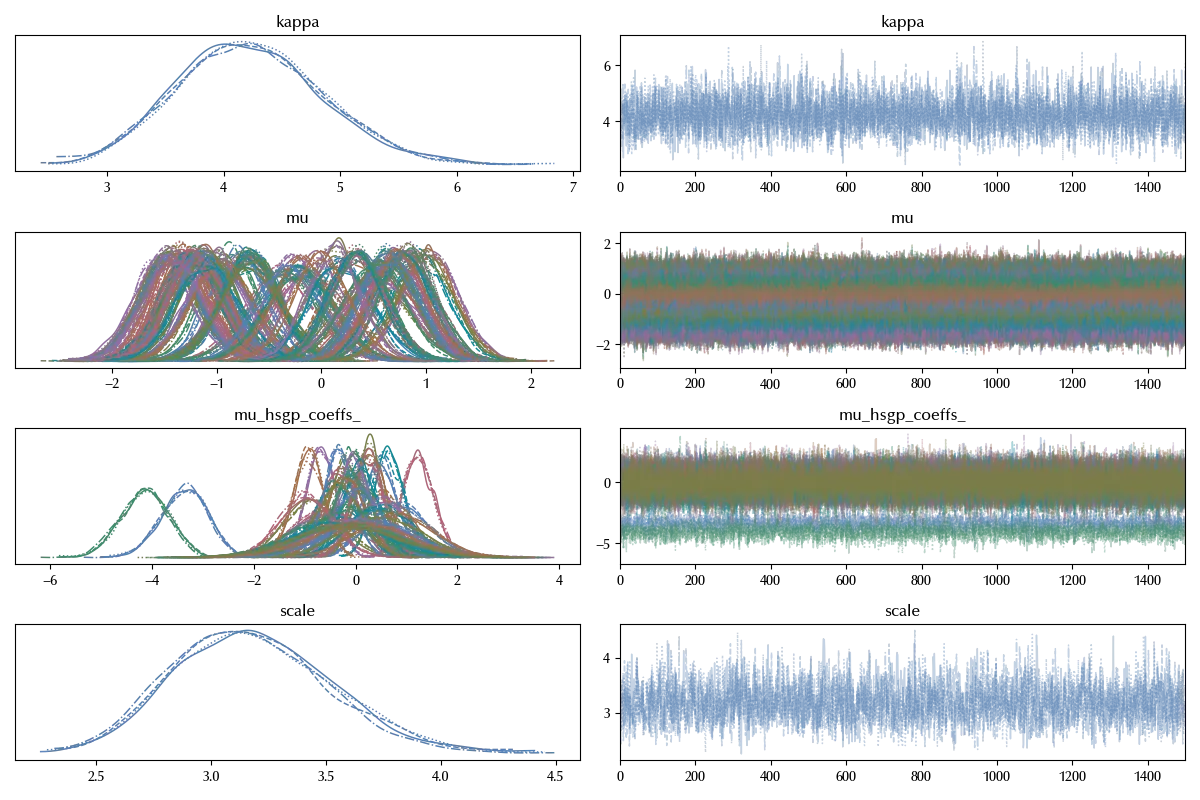
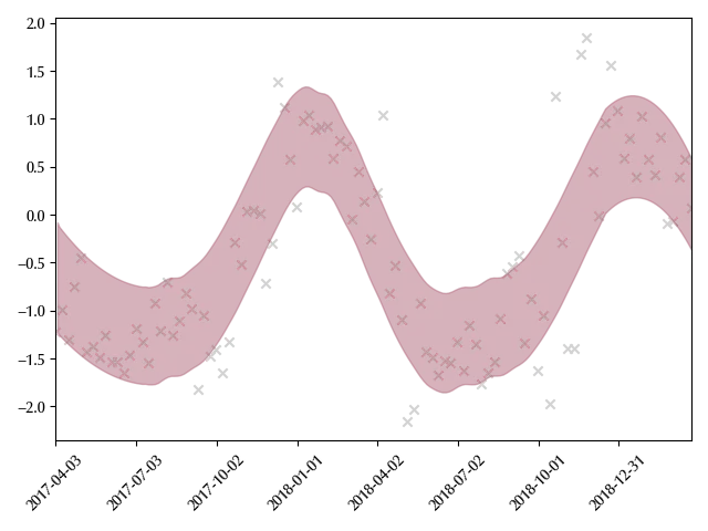
The trace does not show any relevant issue, so we can take a look at our fit.

fig, ax = plt.subplots()
ax.scatter(df_g['X'], df_g['phi'], color='lightgray', marker='x')
az.plot_hdi(df_g['X'], idata_gp.posterior['mu'], ax=ax)
ax.set_xlim([0, df_g['X'].max()])
xticks = ax.get_xticks()
labels = df_g.iloc[[np.argmin(np.abs(df_g['X'].values-elem)) for elem in xticks]]['Date'].dt.strftime('%Y-%m-%d')
ax.set_xticklabels(labels, rotation=45)
fig.tight_layout()

Conclusions

We have seen an easy way to fit circular quantities in PyMC by using the Von Mises distribution, as well as how to encode periodicity in a regression problem by using the Hilbert Space Periodic GP.

Wind direction analysis

GP regression

Conclusions

Suggested readings