

Prior sensitivity analysis
A proper quantification of the impact of the priors on the results is crucial in order to understand the robustness of your conclusions. Everybody knows that, but this idea is often forgotten, and in many results the effect of the priors is simply assumed as negligible. Re-running your model with different priors can be really time-consuming, and up to few years ago the only way to save time was to use conjugate priors. A new fast method to perform this task has however been recently proposed by Kallioinen et al., and this has been soon implemented in Arviz.
The idea is to replace the priors $p(\theta)$, as well as the likelihood $p( y \vert \theta)$, with $p(\theta)^\alpha$ and $p(y \vert \theta)^\alpha$ respectively, with $\alpha \approx 1$. By using a perturbative approach, the impact of the prior can be analytically computed, and we only need to compute the prior or to sample it (or to compute the log-likelihood) in order to perform the sensitivity analysis.
We will use the body fat dataset, that we previously introduced in this previous post, to show how to do this. While in that post we only limited the analysis to few rows, this time we will include all the 252 rows in the analysis.
import numpy as np
import pandas as pd
import pymc as pm
import arviz as az
import arviz_plots as azp
import seaborn as sns
from matplotlib import pyplot as plt

rng = sum(map(ord, 'sensitivity'))

df_bf = pd.read_csv('http://jse.amstat.org/datasets/fat.dat.txt', header=None, sep=r"\s+")

df_bf.columns = ["case", "brozek", "siri",
                                    "density", "age",
                                    "weight_lbs",
                                    "height_in", "bmi",
                                    "fat_free_weight", "neck_cm",
                                    "chest_cm", "abdomen_cm",
                                    "hip_cm", "thigh_cm",
                                    "knee_cm", "ankle_cm",
                                    "biceps_cm", "forearm_cm",
                                    "wrist_cm"]
yobs = df_bf['brozek']

X = df_bf[cols]

with pm.Model(coords={'ind': X.index, 'col': X.columns}) as model:
    sigma = pm.HalfNormal('sigma', sigma=100)
    gamma = pm.Normal('gamma', mu=0, sigma=100)
    beta = pm.Normal('beta', mu=0, sigma=100, dims=['col'])
    mu = gamma + pm.math.dot(beta, X.T)
    y = pm.Normal('y', mu=mu, sigma=sigma, observed=yobs)

with model:
    idata = pm.sample(nuts_sampler='nutpie', draws=2000, tune=2000, random_seed=rng, target_accept=0.9)

az.plot_trace(idata)
fig = plt.gcf()
fig.tight_layout()
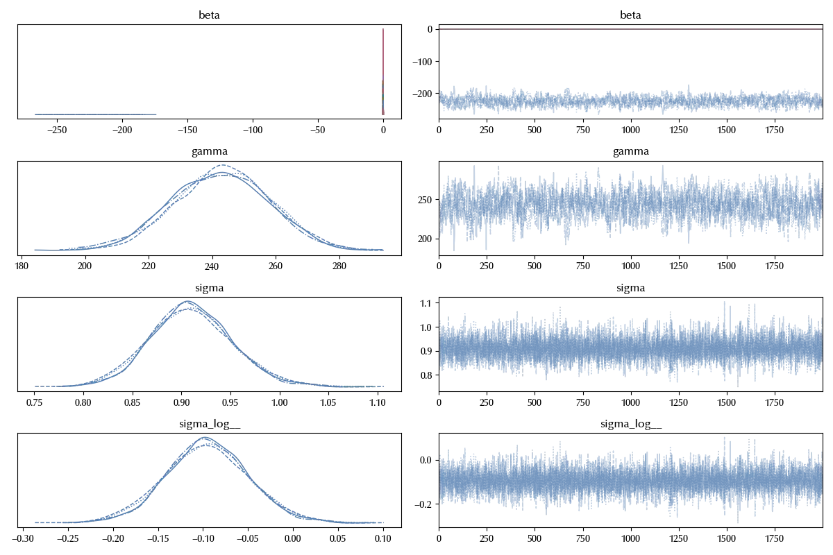
As a general recommendation, avoid using alpha as a parameter name when you plan a sensitivity analysis, since this would conflict with the hidden scale parameter name used by Arviz. The trace seems fine, as there are no divergences or other issues. Let us now inspect the posterior predictive
with model:
    idata.extend(pm.sample_posterior_predictive(idata))

fig, ax = plt.subplots(nrows=4, ncols=4, figsize=(13, 13))
for k, col in enumerate(cols):
    i = k // 4
    j = k % 4
    az.plot_hdi(df_bf[col], idata.posterior_predictive['y'], ax=ax[i][j])
    ax[i][j].scatter(df_bf[col], yobs, marker='x', alpha=0.3, color='lightgray')
    ax[i][j].set_title(col)
fig.tight_layout()
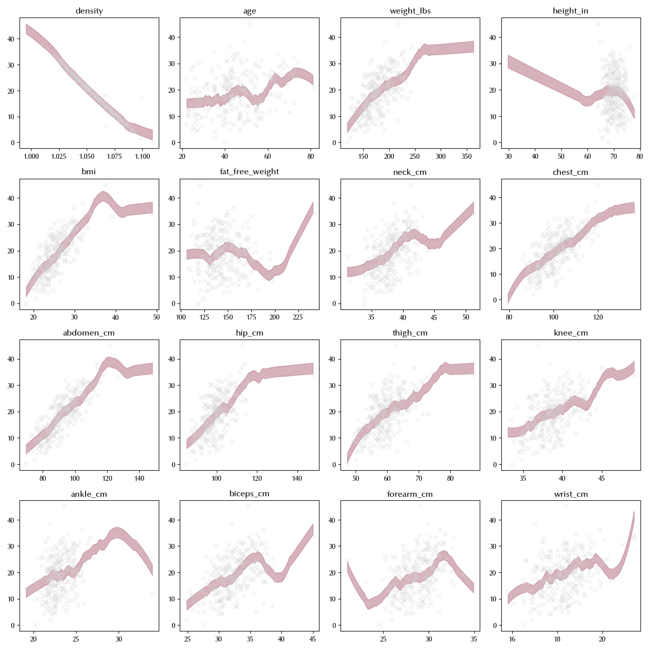
We can see that most of the data lies outside from the HDI region, so we are not correctly reproducing the observed overdispersion. Let us now use sensitivity analysis to better understand the reasons for this.
with model:
    idata.extend(pm.compute_log_prior(idata))

with model:
    idata.extend(pm.compute_log_likelihood(idata))

psens = az.psens(idata)

psens[['beta', 'gamma', 'sigma']].to_dataframe()
| col | beta | gamma | sigma |
|---|---|---|---|
| density | 0.102529 | 0.0994824 | 0.00703698 |
| age | 0.00230812 | 0.0994824 | 0.00703698 |
| weight_lbs | 0.0545761 | 0.0994824 | 0.00703698 |
| height_in | 0.014127 | 0.0994824 | 0.00703698 |
| bmi | 0.0177693 | 0.0994824 | 0.00703698 |
| fat_free_weight | 0.0845982 | 0.0994824 | 0.00703698 |
| neck_cm | 0.00586237 | 0.0994824 | 0.00703698 |
| chest_cm | 0.0147927 | 0.0994824 | 0.00703698 |
| abdomen_cm | 0.0255313 | 0.0994824 | 0.00703698 |
| hip_cm | 0.00286968 | 0.0994824 | 0.00703698 |
| thigh_cm | 0.0202005 | 0.0994824 | 0.00703698 |
| knee_cm | 0.0108598 | 0.0994824 | 0.00703698 |
| ankle_cm | 0.0165331 | 0.0994824 | 0.00703698 |
| biceps_cm | 0.0149032 | 0.0994824 | 0.00703698 |
| forearm_cm | 0.0152033 | 0.0994824 | 0.00703698 |
| wrist_cm | 0.00261026 | 0.0994824 | 0.00703698 |
There are few large values, where large here means greater than the recommended threshold of 0.05 1. This means that the power scale transform of the prior has a large effect of the posterior estimate. We can show this as follows:
azp.plot_psense_dist(idata)
fig = plt.gcf()
fig.tight_layout()
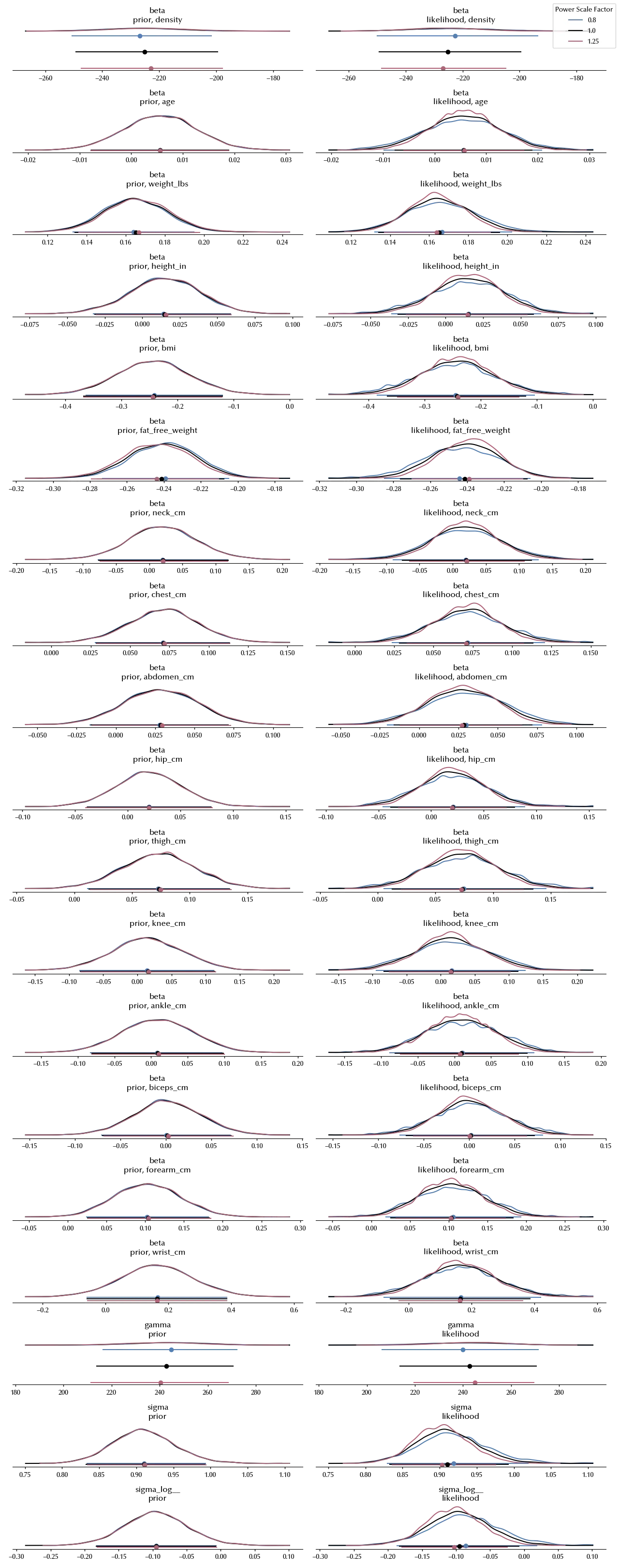
We can see that there’s quite a large effect of the density effect, as well as on gamma. An alternative way to visually inspect the effect is the following one
azp.plot_psense_quantities(
    idata,
    var_names=["gamma", 'sigma'],
    quantities=["mean", "sd", "0.25", "0.75"],
)
fig = plt.gcf()
fig.tight_layout()
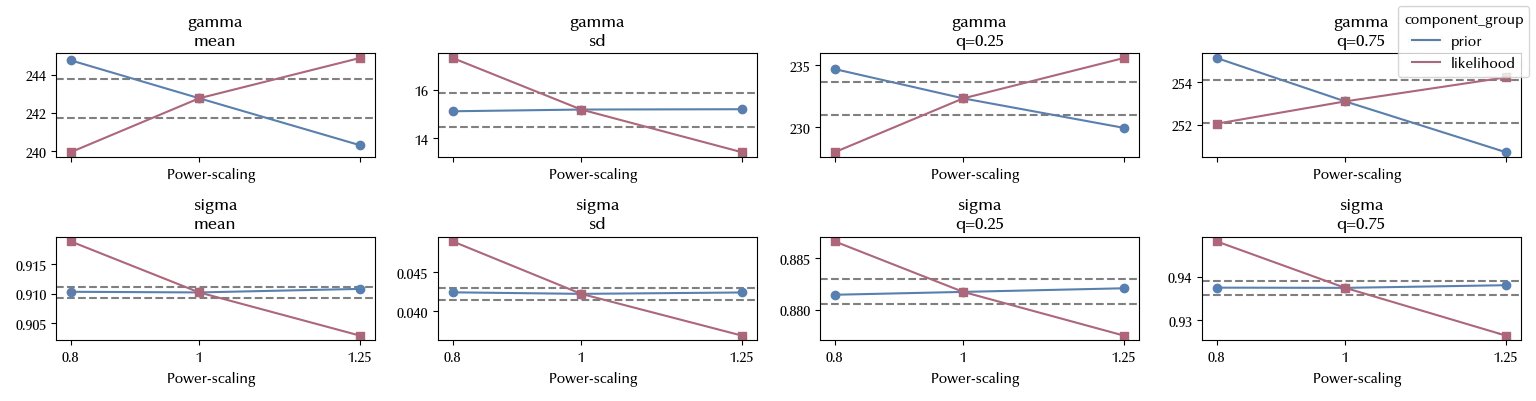
The above analysis tells us that we have an issue, but it does not tell us anything about the causes. We can however easily understend them by comparing the posterior with the prior, and we can either do this by inspecting the trace or, and this is my recommended way to do so, as follows
azp.plot_prior_posterior(
    idata,
    var_names=['beta', 'gamma', 'sigma'],
)
fig = plt.gcf()
fig.tight_layout()
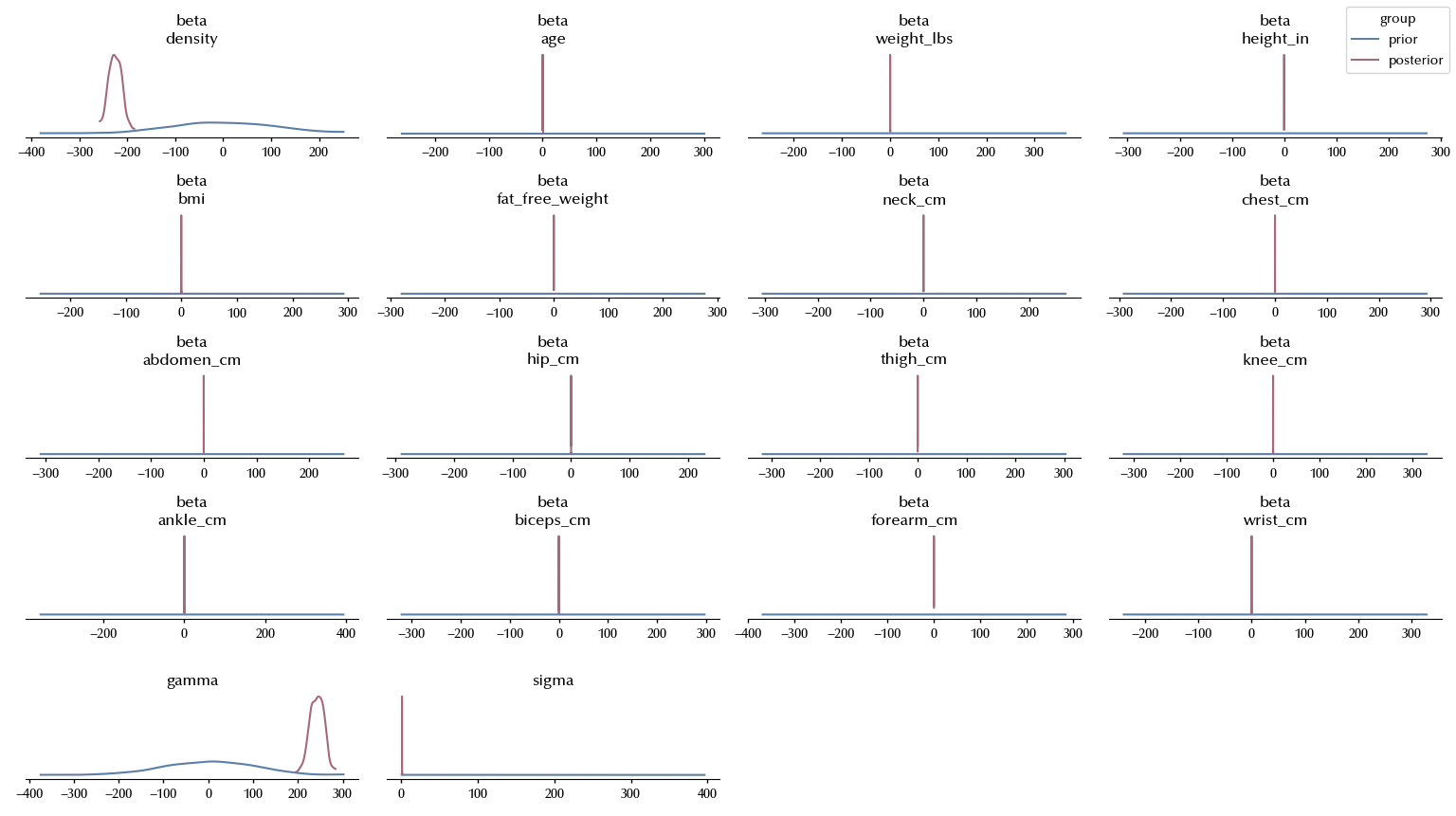
As you can see, most of the posterior mass of the density effect falls away from the center of the prior, and the same holds for gamma.
Conclusions
We have seen how sensitivity analysis as well as prior-posterior comparison can help us in spotting bad prior choice.
- Kallioinen, N., Paananen, T., Bürkner, PC. et al. Detecting and diagnosing prior and likelihood sensitivity with power-scaling. Stat Comput 34, 57 (2024). https://doi.org/10.1007/s11222-023-10366-5
%load_ext watermark
%watermark -n -u -v -iv -w -p xarray,pytensor,nutpie,numpyro,jax,jaxlib
Python implementation: CPython
Python version : 3.13.9
IPython version : 9.7.0
xarray : 2025.1.2
pytensor: 2.35.1
nutpie : 0.16.2
numpyro : 0.19.0
jax : 0.8.0
jaxlib : 0.8.0
arviz_plots: 0.6.0
pymc : 5.26.1
arviz : 0.23.0.dev0
numpy : 2.3.4
matplotlib : 3.10.7
pandas : 2.3.3
seaborn : 0.13.2
Watermark: 2.5.0
-
I generally prefer a smaller threshold of 0.01 in order to keep myself safer, but 0.05 is fine. ↩