Horseshoe priors

When you perform multilinear regression with many independent variables, having highly correlated regressors might have the undesired drawback that most of the associated parameters are barely different from zero. As an example, you might want to find an approximation for some quantity, and you want to include as fewer regressors as possible, maybe because measuring each of them requires effort. Alternatively, if your aim is to assess the impact of some regressor on your model, the instabilities originated by multi-collinearity might lead you to drawing wrong conclusions.

In the frequentist framework, this issue is generally solved by adding regularizing priors, as in the case of LASSO regression. In the Bayesian one, the natural way to overcome this problem is by means of an appropriate choice of the priors for the regressors, and the Bayesian community proposed the family of sparsifying priors. Here we will only discuss the horseshoe prior, but many more have been proposed, and we will provide some link the topic.

The Body Fat dataset

In this example, we will use the Body Fat dataset, which is discussed in this blog.

The body fat percentage is the mass of the fat of the body divided by the total mass. This quantity can be accurately estimated by using some dedicated instrument, which are however time-consuming and require some knowledge in order to be used. In order to have a less precise measurement, we can try and estimate it by relating it to some other quantity which is easier to perform, such as weight or length measurements. While it is reasonable to use the body weight, it is however less clear which length measurement we should use in order to find a good proxy for the desired quantity. We could use the total height, but we could also use many more length measurements, such as the neck circumference or the abdomen one.

A starting point can be to use a multilinear regression in order to find out which quantity better predicts the body fat percentage. However, a more robust person will have large values for all of them, we can therefore expect that our dataset will show a quite strong multicollinearity.

import numpy as np
import pandas as pd
import pymc as pm
import arviz as az
import seaborn as sns
from matplotlib import pyplot as plt

rng = np.random.default_rng(42)

df_bf = pd.read_csv('http://jse.amstat.org/datasets/fat.dat.txt', header=None, sep=r"\s+")

df_bf.columns = ["case", "brozek", "siri", 
                                    "density", "age", 
                                    "weight_lbs", 
                                    "height_in", "bmi", 
                                    "fat_free_weight", "neck_cm", 
                                    "chest_cm", "abdomen_cm", 
                                    "hip_cm", "thigh_cm", 
                                    "knee_cm", "ankle_cm", 
                                    "biceps_cm", "forearm_cm",
                                    "wrist_cm"]

There are at least two formulas to estimate the body fat percentage, and we will use the “Brozek” formula.

df.head()

	case	brozek	siri	density	age	weight_lbs	height_in	bmi	fat_free_weight	neck_cm	chest_cm	abdomen_cm	hip_cm	thigh_cm	knee_cm	ankle_cm	biceps_cm	forearm_cm	wrist_cm
0	1	12.6	12.3	1.0708	23	154.25	67.75	23.7	134.9	36.2	93.1	85.2	94.5	59	37.3	21.9	32	27.4	17.1
1	2	6.9	6.1	1.0853	22	173.25	72.25	23.4	161.3	38.5	93.6	83	98.7	58.7	37.3	23.4	30.5	28.9	18.2
2	3	24.6	25.3	1.0414	22	154	66.25	24.7	116	34	95.8	87.9	99.2	59.6	38.9	24	28.8	25.2	16.6
3	4	10.9	10.4	1.0751	26	184.75	72.25	24.9	164.7	37.4	101.8	86.4	101.2	60.1	37.3	22.8	32.4	29.4	18.2
4	5	27.8	28.7	1.034	24	184.25	71.25	25.6	133.1	34.4	97.3	100	101.9	63.2	42.2	24	32.2	27.7	17.7

We will use only a subset of variables as regressors, and in order to make evident the effect of the multicollinearity, we will only use the first 40 measurements.

indx = [5, 6, 11, 12, 13, 14, 15, 16, 17, 18]

df = df_bf.iloc[:40]

yobs = df['brozek']/100

X = df[df.columns[indx]]

Xnorm = (X-np.mean(X, axis=0))/np.std(X, axis=0)/2

sns.pairplot(Xnorm)

The pairplot of the regressors

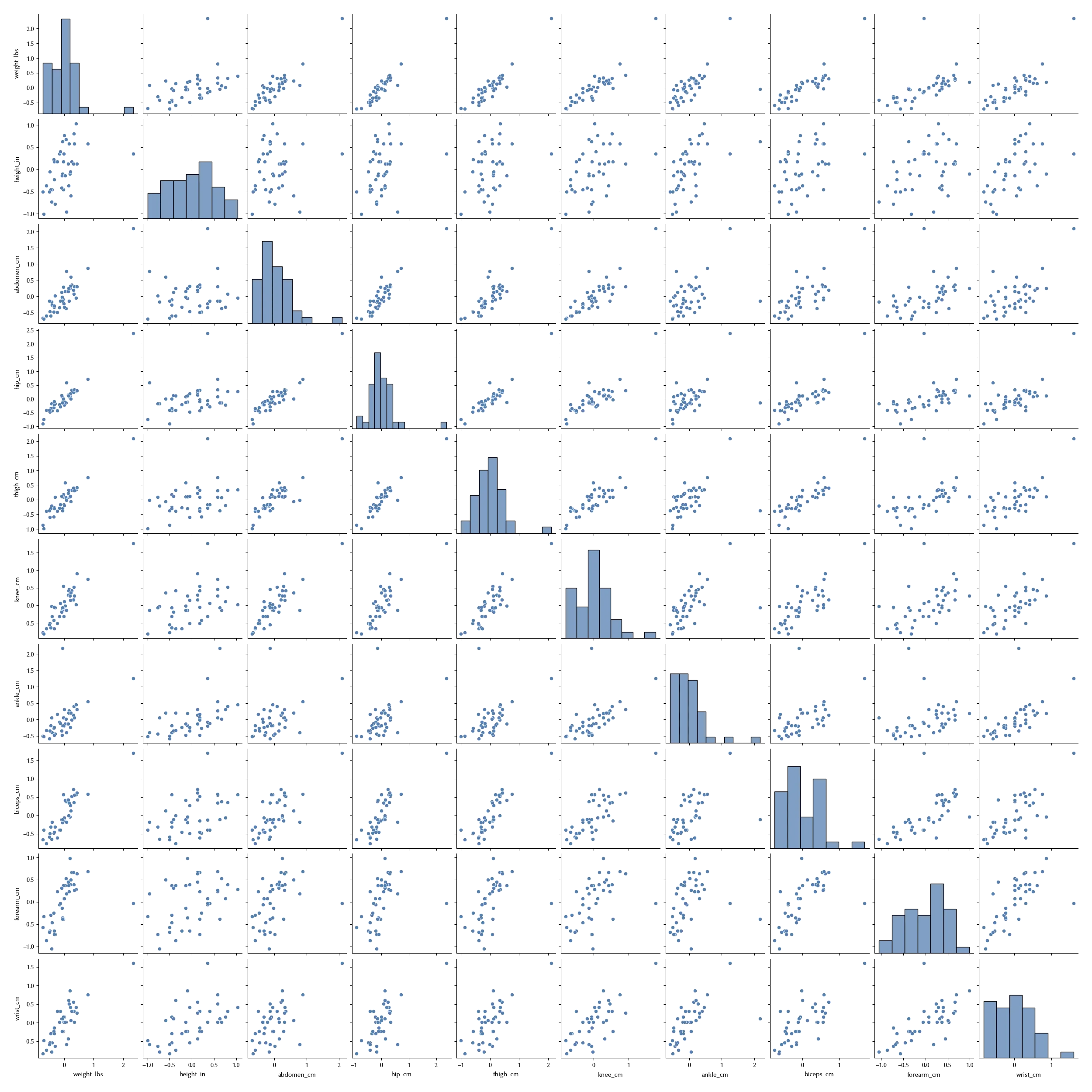
As you can see by the above plot, the regressors dataset shows a pronounced multi-collinearity, since they are not pairwise-independent. In order to facilitate the comparison across coefficients, we will use the (Gelman’s version of the) standardized coefficients. Since the choice of a suitable scale for the prior is very important, we scaled the observation by a factor 100, and in this way the target variable ranges from 0 to 1.

Let us first try and see what happens if we only include one variable into a linear regression model.

starting_models = []
for i in range(len(X.columns)):
    with pm.Model() as mod:
        alpha = pm.Normal('alpha', sigma=1000)
        sigma = pm.HalfNormal('sigma', sigma=1000)
        beta = pm.Normal('beta', mu=0, sigma=1000)
        mu = alpha + beta*Xnorm[X.columns[i]]
        y = pm.Normal('y', mu=mu, sigma=sigma, observed=yobs)
        idata = pm.sample(nuts_sampler='numpyro', random_seed=rng)
        # pm.compute_log_likelihood(idata)
        # idata.extend(pm.sample_posterior_predictive(idata, random_seed=rng))
        starting_models.append([{'vars': [X.columns[i]], 'model': mod, 'idata': idata}])

traces = [model[0]['idata'] for model in starting_models]
names = [model[0]['vars'][0] for model in starting_models]

fig, ax = plt.subplots(figsize=(5, 9))
az.plot_forest(traces, model_names=names, var_names=['beta'], combined=True, ax=ax)
ax.axvline(x=0, ls=':', color='lightgray')

The forest plot for
the regression coefficients across the different models

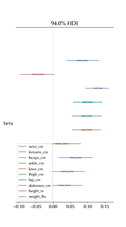
From the above credible intervals, we conclude that height_in, ankle_cm, forearm_cm are wrist_cm compatible with 0. Let us include all except these variables into a multilinear regression.

indx_pos = [k for k, trace in enumerate(traces)
            if (az.summary(trace, var_names=['beta'])['hdi_3%']*az.summary(trace, var_names=['beta'])['hdi_97%']).values[0]>0]

Xtmp = Xnorm[[X.columns[k] for k in indx_pos]]

with pm.Model(coords={'cols': Xtmp.columns, 'idx': Xtmp.index}) as model_2:
        alpha = pm.Normal('alpha', sigma=1000)
        sigma = pm.HalfNormal('sigma', sigma=1000)
        beta = pm.Normal('beta', mu=0, sigma=1000, dims=['cols'])
        mu = alpha + pm.math.dot(beta, Xtmp.T)
        y = pm.Normal('y', mu=mu, sigma=sigma, observed=yobs)

with model_2:
    idata_2 = pm.sample(nuts_sampler='numpyro', random_seed=rng)

az.plot_trace(idata_2)
fig = plt.gcf()
fig.tight_layout()

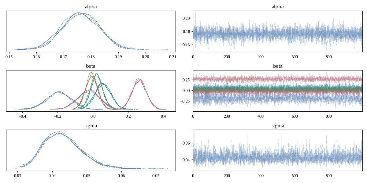
We only have few non-zero regression coefficients:

fig, ax = plt.subplots(figsize=(5, 4))
az.plot_forest(idata_2, var_names=['beta'], ax=ax, combined=True)
ax.axvline(x=0, ls=':', color='lightgray')

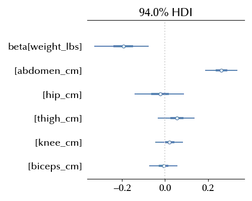
Only two of them appear to be different from zero. This kind of iterative procedure to prune away the irrelevant variables is a possible way to proceed. At this point, we could only include weight and abdomen, and maybe include one more regressor per time. This is however both time-consuming and questionable: one might ask why did you proceed in such an order, and whether using a different order might have changed the result. Let us as an example start by using all the variables.

with pm.Model(coords={'ind': X.index, 'col': X.columns}) as model:
    sigma = pm.HalfNormal('sigma', sigma=1000)
    alpha = pm.Normal('alpha', mu=0, sigma=1000)
    beta = pm.Normal('beta', mu=0, sigma=1000, dims=['col'])
    mu = alpha + pm.math.dot(beta, Xnorm.T)
    y = pm.Normal('y', mu=mu, sigma=sigma, observed=yobs)

with model:
    idata = pm.sample(nuts_sampler='numpyro', draws=5000, tune=5000, random_seed=rng, target_accept=0.9)

az.plot_trace(idata)
fig = plt.gcf()
fig.tight_layout()

The trace of the full model

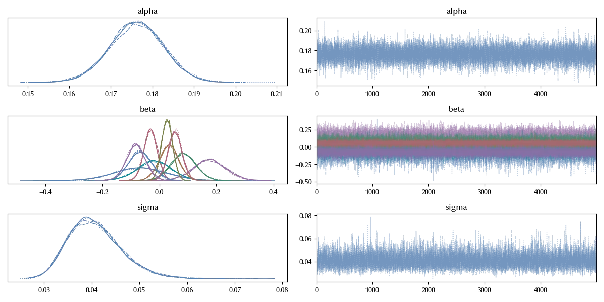
fig = plt.figure(figsize=(6, 10))
ax = fig.add_subplot(111)
az.plot_forest(idata, var_names=['beta'], ax=ax)
ax.axvline(x=0, color='lightgrey', ls=':')
fig.tight_layout()

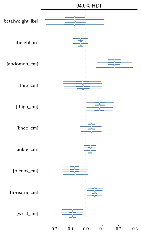
As you can see, we would have a different result.

As previously anticipated, there is an alternative way to proceed, and is by using an appropriate set of priors. A reasonable choice is given by

\[\begin{align} \beta_i \sim & \mathcal{N}(0, \sigma \tau_i)\\ \tau_i \sim & \mathcal{HalfCauchy}(0, 1)\\ \end{align}\]

The reason for this is quite simple: the half-Cauchy distribution has a large amount of mass close to zero, but it also has fat tails. In this way, the posterior is either shrunk to zero, or far away from zero, and intermediate results are somehow “discouraged” by the prior.

How to properly choose $\sigma$ is not trivial, and a recommended choice is

\[\sigma \sim \mathcal{HalfCauchy}(0, a)\]

A large value of $a$ will not strongly affect the posterior, while a small value will shrink the posterior to 0. In our case, we choose $a=1\,,$ which is quite a large value if we compare it to the expected effect of the regression coefficients. We leave to the reader the sensitivity analysis of the inference depending on the choice of $a$. You should keep in mind that your conclusions might strongly depend on the choice of $a$, so in this case a proper sensitivity analysis is strongly recommended.

with pm.Model(coords={'ind': X.index, 'col': X.columns}) as model_hh:
    sigma = pm.HalfNormal('sigma', sigma=1000)
    alpha = pm.Normal('alpha', mu=0, sigma=1000)
    sig_beta = pm.HalfCauchy('sig_beta', beta=1, dims=['col'])
    sig = pm.HalfCauchy('sig', 1)
    mu_beta = pm.Normal('mu_beta', mu=0, sigma=100)
    beta = pm.Deterministic('beta', mu_beta+sigma*sig_beta, dims=['col'])
    mu = alpha + pm.math.dot(beta, Xnorm.T)
    y = pm.Normal('y', mu=mu, sigma=sigma, observed=yobs, dims=['ind'])

with model_hh:
    idata_hh = pm.sample(nuts_sampler='numpyro', draws=5000, tune=5000, random_seed=rng, target_accept=0.9)

az.plot_trace(idata_hh)
fig = plt.gcf()
fig.tight_layout()

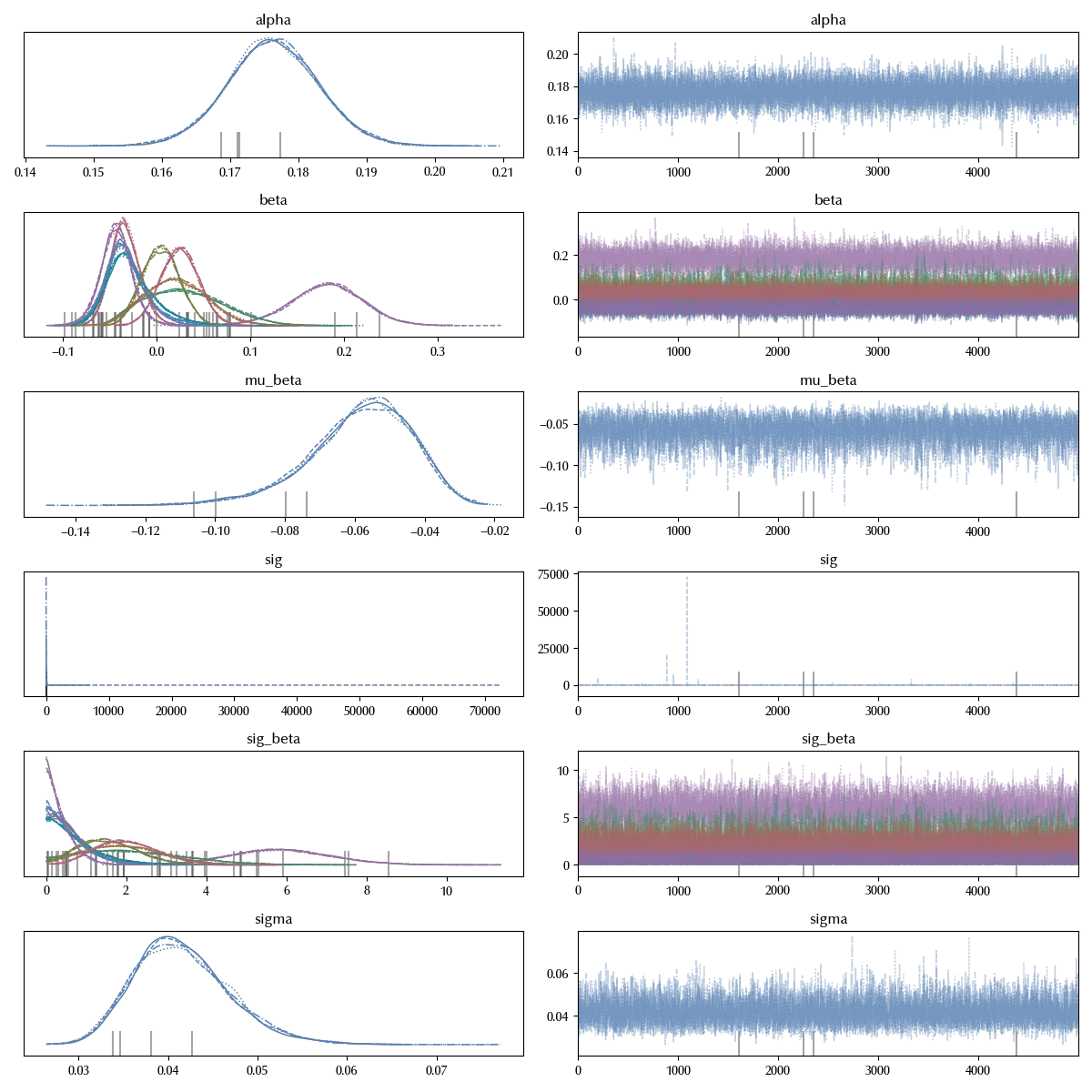
fig = plt.figure(figsize=(6, 10))
ax = fig.add_subplot(111)
# az.plot_forest({'std': idata, 'hh': idata_hh}, var_names=['beta'], ax=ax, model_names=['std', 'hh'])
az.plot_forest([idata, idata_hh], var_names=['beta'], ax=ax, model_names=['std', 'hh'], combined=True)
ax.axvline(x=0, color='lightgrey', ls=':')
fig.tight_layout()

We can now compare the forest plot of the two models containing all the variables.

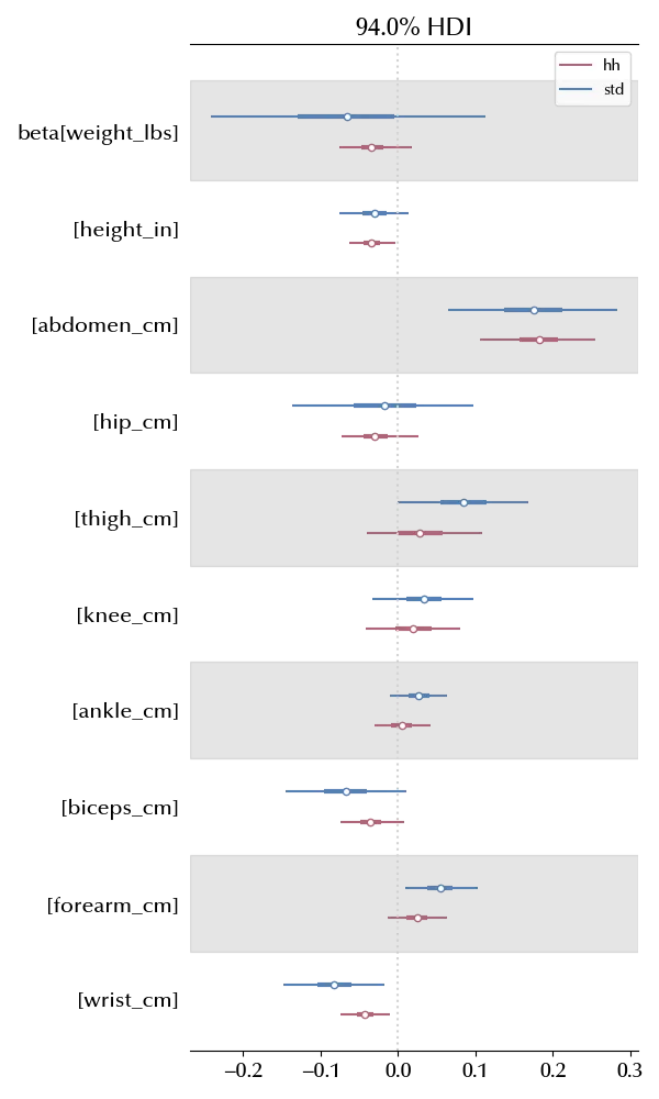
The error bars of the horseshoe model are much smaller than the ones of the standard model, and the net result of using the horseshoe is that the posterior distribution of the regression coefficients are more sparse than the ones of the standard multilinear model. If you perform a sensitivity analysis, you should obtain the same results for quite a large range of choices for the scale parameter.

Conclusions

We have seen how an appropriate choice of the prior distribution allows us to enforce sparsity in the regression coefficients of a multilinear model. There are of course other possible approach to the problem, such as factor analysis or only adding one regressor per time, as we did in the beginning. However, according to my own view, an appropriate choice of the prior to enforce some desired condition is the best way to leverage the Bayesian workflow to tackle any issue, including multi-collinearity.

The Body Fat dataset

Conclusions

Suggested readings