Randomized controlled trials

As we anticipated in the last post, when we have randomization, association implies causation. In this case we can use a simple regression model to assess if the treatment causes an effect.

Randomized controlled trials are the golden standards in clinical studies, but they are widely used in other fields like industry or marketing campaigns. Thanks to their popularity, even marketing providers such as Mailchimp allow you to easily implement this kind of studies, and in this post we will see how to analyze them by using Bayesian regression. In this experiment we will analyze the data from a newsletter, and what we will determine is whether the presence of the first name (which is required in the login form) in the mail preview increases the probability of opening the email. When we programmed the newsletter, we divided the total audience into two blocks, and each recipient has been randomly assigned to one block. In the control block (t=0) we sent the email without the first name in the mail preview, while to the other recipients we sent the email with the first name in the mail preview.

Some mails were bounced, but at the end $n_t = 2326$ users received the test mail and $n_c = 2347$ received the control mail. $y_t = 787$ users out of 2326 opened the test email, while $y_c=681$ users out of 2347 opened the control one.

Since the opening action is a binary variable, we will take a binomial likelihood. We will therefore use a logistic regression to estimate the ATE.

\[\begin{align} & y_{c} \sim \mathcal{Binom}(p_c, n_n) \\ & y_{t} \sim \mathcal{Binom}(p_t, n_t) \\ & p_c = \frac{1}{1+e^{-\beta_0}} \\ & p_t = \frac{1}{1+e^{-(\beta_0+ \beta_1)}} \end{align}\]

We will take the default Bambi prior, which is considered weakly informative, for both parameters.

We can now easily implement our model in Bambi

import pandas as pd
import pymc as pm
import arviz as az
import bambi as pmb
import numpy as np
from matplotlib import pyplot as plt

random_seed = np.random.default_rng(42)

n_t = 2326
n_c = 2347

k_t = 787
k_c = 681

grp = [0]*n_c + [1]*n_t
ks = [1]*k_c + [0]*(n_c-k_c) + [1]*k_t + [0]*(n_t-k_t)

df = pd.DataFrame({'g': grp, 'k': ks})

model = pmb.Model('k ~ g', data=df, family="bernoulli")

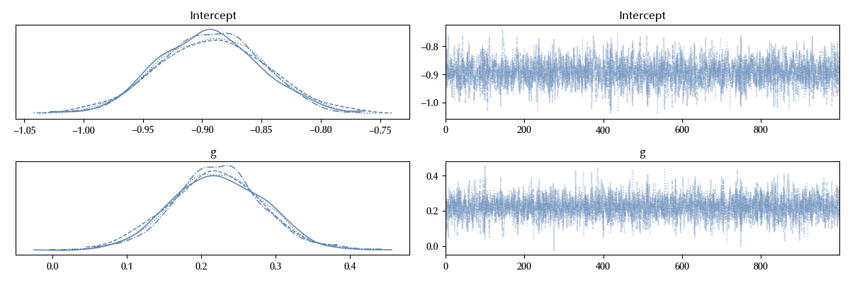
idata = model.fit(nuts_sampler='numpyro')

az.plot_trace(idata)
fig = plt.gcf()
fig.tight_layout()

The trace of our model

We can now compute the average treatment effect

def invlogit(x):
    return 1/(1+np.exp(-x))

# We compute the probability for a control group email of being opened
pc = invlogit(idata.posterior['Intercept'].values).reshape(-1)

# We compute the probability for a test group email of being opened
pt = invlogit(idata.posterior['Intercept'].values + idata.posterior['g'].values).reshape(-1)

ate = pt - pc

fig, ax = plt.subplots()
az.plot_posterior(ate, ax=ax)
ax.set_title('ATE')
fig.tight_layout()

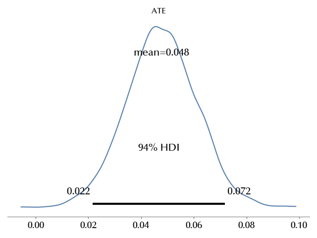
The posterior distribution for the average treatment effect

The ATE looks positive with a probability close to 1

(ate>0).mean()

0.9995

We are almost sure that, in our test, using the first name in the mail preview increased the opening probability of the newsletter.

Notice that we restricted our discussion to one single newsletter, and we avoided more general claims regarding future newsletters we will send. However, we have some indication that our audience may prefer more personal newsletters.

Conclusions

We saw an example of how to perform causal inference in Bayesian statistics for randomized controlled experiments by using regression models in PyMC. We also discussed the proper interpretation of the results.

Conclusions

Suggested readings