Instrumental variable regression

In many circumstances you cannot randomize, either because it is unethical or simply because it’s too expensive. There are however methods which, if appropriately applied, may provide you some convincing causal evidence.

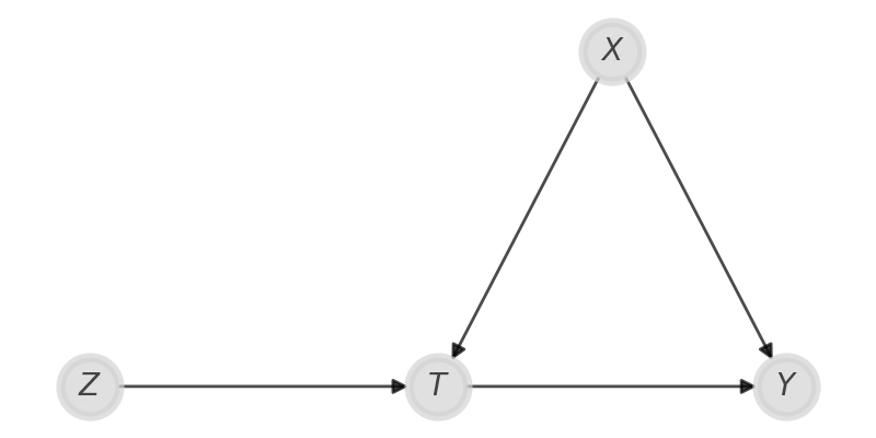
Let us consider the case where you cannot randomly assign the treatment $T\,,$ and in this case it could be affected by any confounder $X$ leading you to a biased estimate of the treatment effect. However, if you have a variable $Z$ that only affects $T$ and does not affect your outcome in any other way other than via $T\,,$ than you can apply Instrumental Variable Regression.

The assumed causal flow

Of course, the above causal assumption is quite strong, but it holds in quite a good approximation in some circumstance.

This method has been applied to analyze the effect of school years ($T$) on earning ($Y$). In this case the variable $Z$ was the assignment of some monetary assistance (a voucher) to go to school.

One would be tempted to simply use linear regression to fit this model:

\[Y = \alpha + \beta T + \gamma Z + \varepsilon\]

However, linear regression assumes independence between the regressors, while in our case we have that $T$ is determined by $Z\,.$ This has an impact on the variance estimate of $Y\,,$ as we do not correctly propagate the uncertainty due to the $T$ dependence on $Z\,.$ In fact, linear regression always predicts homoscedastic variance, while IV can also reproduce heteroscedasticity.

The model we used here is an adaptation of the one provided in this page.

Application to the cigarettes sales

We will use IV to see if an increase in the cigarettes price ($T$) causes a decrease in the cigarettes sales ($Y$), and we will use the tobacco taxes as instrumental variable $Z$. In order to linearize the dependence between the variables, instead of the value of each quantity, we will consider the difference between the 1995 log value and the 1985 log value.

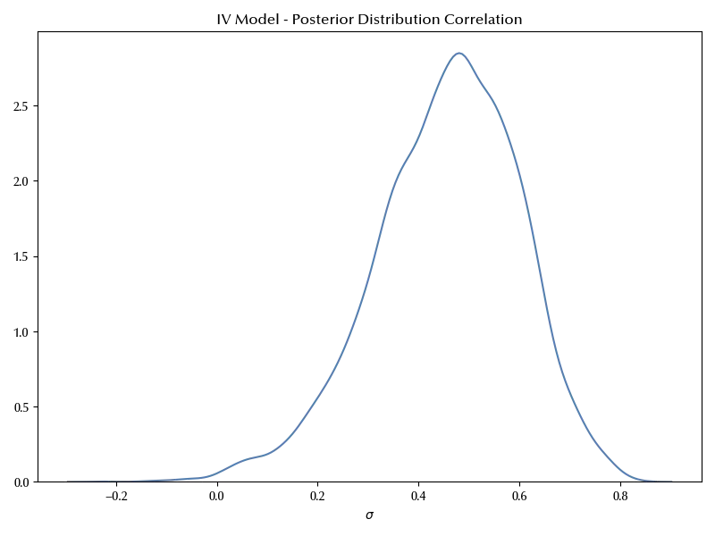
\[\begin{pmatrix} T \\ Y \\ \end{pmatrix} \sim \mathcal{t} \left( \left( \alpha_0 + \beta_0 Z \atop \alpha_1 + \beta_1 T \right), \Sigma, \nu \right)\]

where $t$ represents the 2 dimensional Student-T distribution and $\Sigma$ is the $2\times2$ covariance matrix. If $Z$ has a causal effect on $Y$ via $T\,,$ then the correlation between $Y$ and $T$ is different from zero.

We will assume

\[\alpha_i, \beta_i \sim \mathcal{N}(0, 10^3)\]

and

\[\nu \sim \mathcal{HalfNormal}(100)\]

$\Sigma$ must be a positive semi-defined matrix, and an easy way to provide it a prior is using the Lewandowski-Kurowicka-Joe distribution . This distribution takes a shape parameter $\eta\,,$ and we will take $\eta=1\,,$ which implies that we will take a uniform prior over $[-1, 1]$ for the correlation matrix. We will moreover assume that the standard deviations are distributed according to

\[\sigma_i \sim \mathcal{HalfCauchy}(20)\]

import pandas as pd
import numpy as np
import pymc as pm
import arviz as az
import seaborn as sns
from matplotlib import pyplot as plt
from pytensor.tensor.extra_ops import cumprod

random_seed = np.random.default_rng(42)

df_iv = pd.read_csv('https://raw.githubusercontent.com/vincentarelbundock/Rdatasets/master/csv/AER/CigarettesSW.csv')

X_iv = (np.log(df_iv[df_iv['year']==1995]['price'].values)
        - np.log(df_iv[df_iv['year']==1985]['price'].values)
       )/np.log(df_iv[df_iv['year']==1985]['price'].values)
Y_iv = (np.log(df_iv[df_iv['year']==1995]['packs'].values)
        - np.log(df_iv[df_iv['year']==1985]['packs'].values)
       )/np.log(df_iv[df_iv['year']==1985]['packs'].values)
Z_iv = (np.log(df_iv[df_iv['year']==1995]['taxs'].values)
        - np.log(df_iv[df_iv['year']==1985]['taxs'].values)
       )/np.log(df_iv[df_iv['year']==1985]['taxs'].values)

with pm.Model() as instrumental_variable:
    sd_dist = pm.HalfCauchy.dist(beta=20.0, size=2)
    nu = pm.HalfNormal('nu', sigma=100.0)
    chol, corr, sigmas = pm.LKJCholeskyCov('sigma', eta=1., n=2, sd_dist=sd_dist)
    alpha = pm.Normal('alpha', mu=0, sigma=1000, shape=2)
    beta = pm.Normal('beta', mu=0, sigma=1000, shape=2)
    w = np.stack([Z_iv, X_iv], axis=1)
    u = np.stack([X_iv, Y_iv], axis=1)
    mu = pm.Deterministic('mu', alpha + beta*w)  # so we will recover it easily
    y = pm.MvStudentT('y', mu=mu, chol=chol, nu=nu, shape=(2, len(Y_iv)), observed=u)
    # We directly compute the posterior predictive
    y_pred = pm.MvStudentT('y_pred', mu=mu, chol=chol, nu=nu)

with instrumental_variable:
    trace_instrumental_variable = pm.sample(draws=2000, tune=2000, chains=4, random_seed=random_seed,
                                           nuts_sampler='numpyro')

az.plot_trace(trace_instrumental_variable ,
              var_names=['alpha', 'beta', 'sigma', 'nu'],
              coords={'sigma_corr_dim_0':0, 'sigma_corr_dim_1':1})
fig = plt.gcf()
fig.tight_layout()

The trace plot of the above model

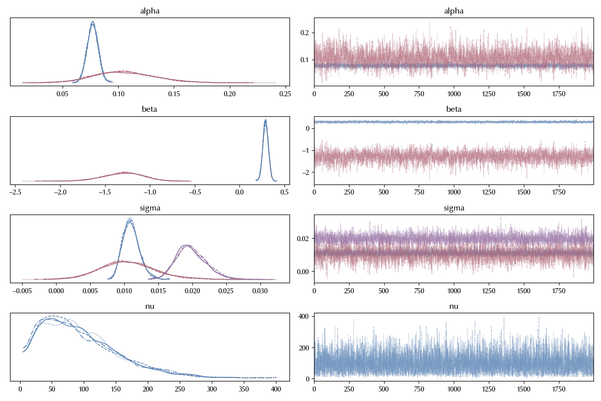
As we can see, there is no signal of problems in thee trace plot.

A few remarks on the above code. Since the model is not very fast, we used the numpyro sampler, which hundred of times faster than the standard PyMC sampler. Moreover, we instructed arviz to only plot the off-diagonal elements of the correlation matrix. We must do this because the diagonal elements are always one, as they must be, but this causes an error in arviz (which assumes a random behavior in all the variables of the trace).

We can now verify the posterior predictive distribution.

a0 = trace_instrumental_variable.posterior['alpha'].mean(dim=['draw', 'chain'])[1].values
b0 = trace_instrumental_variable.posterior['beta'].mean(dim=['draw', 'chain'])[1].values

x_min = 0.06
x_max = 0.2

x_pl = np.arange(x_min, x_max, 0.0002)

xiv_0 = trace_instrumental_variable.posterior['y_pred'].values.reshape((-1, 48, 2))[:, :, 0]
xiv_1 = trace_instrumental_variable.posterior['y_pred'].values.reshape((-1, 48, 2))[:, :, 1]

sampled_index = np.random.randint(low=0, size=100, high=1000)

sampled_index

fig = plt.figure()
ax = fig.add_subplot()
ax.plot(x_pl, a0+b0*x_pl, color='gray', alpha=0.8)
for k in sampled_index:
    ax.scatter(xiv_0[k], xiv_1[k], color='lightgray', marker='x')
ax.scatter(X_iv, Y_iv, color='steelblue', marker='o')
ax.set_ylabel('y', rotation=0)
ax.set_xlabel('t')
ax.set_xlim([x_min, x_max])
fig.tight_layout()

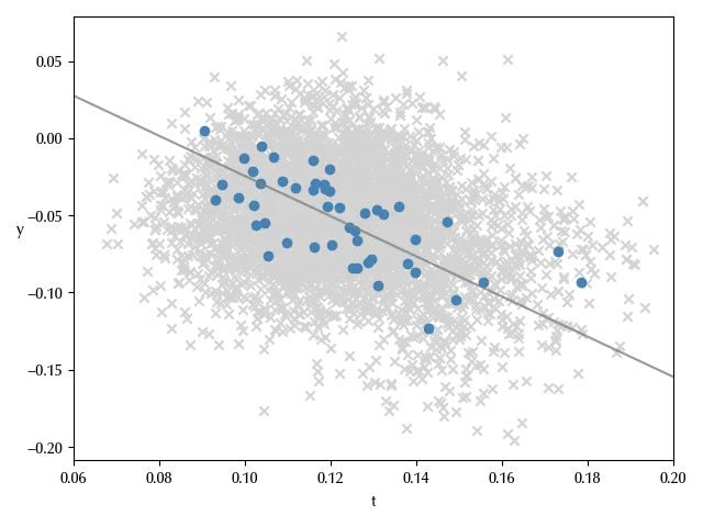
The posterior predictive distribution

Our model also looks capable to reproduce the observed data.

fig, ax = plt.subplots(figsize=(8, 6))
sns.kdeplot(
    x=az.extract(data=trace_instrumental_variable, var_names=["sigma_corr"])[0, 1, :],
    ax=ax,
)
ax.set(title="IV Model - Posterior Distribution Correlation")
ax.set_xlabel(r'$\sigma$')
ax.set_ylabel(r'')
fig.tight_layout()

The off-diagonal component of the correlation matrix

Conclusions

We have seen how IV allows us to make causal inference in absence of randomization, but making some rather strong assumptions about the causal structure of the problem. We have also seen how to implement it in PyMC.

Application to the cigarettes sales

Conclusions

Suggested readings