Regression discontinuity design

Regression Discontinuity Design (RDD) can be applied when there is a threshold above which some causal effect applies, and allows you to infer the impact of such an effect on your population. More precisely, you can determine the average treatment effect on a neighborhood of the threshold. In most countries, there is a retirement age, and you might analyze the impact of the retirement on your lifestyle. There are also countries where school classes has a maximum number of students, and this has been used to assess the impact of the number of students on the students’ performances. Here we will re-analyze, in a Bayesian way, the impact of alcohol on the mortality, as done in “Mastering Metrics”. In the US, at 21, you are legally allowed to drink alcohol, and we will use RDD to assess the impact on this on the probability of death in the US. As the previous model, this one has been implemented in CausalPy too, so you if you are interested in using this model, you should consider running pip install CausalPy.

Implementation

Let us first of all take a look at the dataset.

import pandas as pd
import numpy as np
import pymc as pm
import bambi as pmb
import arviz as az
import seaborn as sns
from matplotlib import pyplot as plt

rng = np.random.default_rng(42)
kwargs = {'nuts_sampler': 'numpyro', 'random_seed': rng,
          'draws': 5000, 'tune': 5000, 'chains': 4, 'target_accept': 0.9}

df_madd = pd.read_csv("https://raw.githubusercontent.com/seramirezruiz/stats-ii-lab/master/Session%206/data/mlda.csv")

fig = plt.figure()
ax = fig.add_subplot(111)
sns.scatterplot(data=df_madd,x='forcing', y='outcome')
ax.axvline(x=0, color='k', ls=':')
fig.tight_layout()

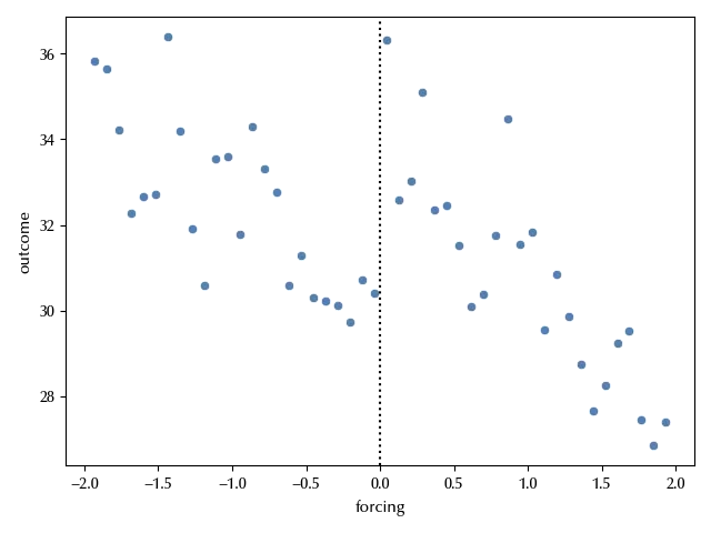
A linear model seems appropriate, and it seems quite clear that there is a jump when the forcing variable (age-21) is zero.

While RDD can be both applied with a sharp cutoff and a fuzzy one, we will limit our discussion to the sharp one. We will take a simple linear model, as polynomial models should be generally avoided in RDD models as they tend to introduce artifacts.

\[y \sim \mathcal{N}( \alpha + \beta x + \gamma \theta(x), \sigma)\]

Here $x$ is the age minus 21, while $\theta(x)$ is the Heaviside theta

\[\theta(x) = \begin{cases} 0 & x\leq0 \\ 1 & x > 0\\ \end{cases}\]

As usual, we will assume a non-informative prior for all the parameters.

df_red = df_madd[['forcing', 'outcome']]

df_red['discontinuity'] = (df_red['forcing']>0).astype(int)

model = pmb.Model('outcome ~ forcing + discontinuity', data=df_red)

idata = model.fit(**kwargs)

az.plot_trace(idata)
fig_trace = plt.gcf()
fig_trace.tight_layout()

The trace looks fine, and it is clear that the value of the discontinuity is quite large.

az.plot_posterior(idata, var_names=['discontinuity'])
fig = plt.gcf()
fig.tight_layout()

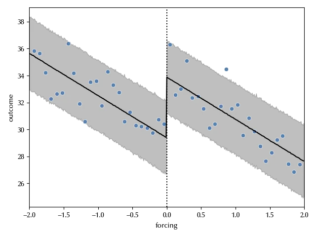
Let us now verify if our model is capable of reproducing the observed data.

x_pl = np.arange(-2, 2, 1e-2)
df_plot = pd.DataFrame({'forcing': x_pl, 'discontinuity': (x_pl>0).astype(int)})

model.predict(idata=idata, data=df_plot, inplace=True, kind='response')

pp_madd = idata.posterior_predictive.outcome.values.reshape((-1, len(x_pl)))

madd_mean = np.mean(pp_madd, axis=0)
fig, ax = plt.subplots()
az.plot_hdi(x=x_pl, y=pp_madd, smooth=False, color='gray', ax=ax, hdi_prob=0.94)
sns.scatterplot(data=df_red,x='forcing', y='outcome')
ax.axvline(x=0, color='k', ls=':')
ax.plot(x_pl, madd_mean, color='k')
ax.set_xlim([-2, 2])
fig.tight_layout()

Conclusions

We re-analyzed the effect of the Minimum Legal Driving Age (MLDA) on the mortality, and we discussed how to apply RDD to perform causal inference in the presence of a threshold.

Before concluding, we would like to warn the reader that applying the RDD design to time series might look appealing, but it’s rarely a good idea. We won’t give you the details for this, and the interested reader is invited to go through this paper by Hausman and Rapson and references therein.

Implementation

Conclusions

Suggested readings