The Gaussian model

In the previous posts we worked with discrete data (either binary or count data).

Before moving to more advanced topic, we will briefly show that dealing with real-valued data only requires to use a real-valued likelihood.

The normal distribution

In order to show how to deal with real-valued data, we will use a well known dataset which is well described by a normal distribution, namely the housefly wing dataset provided at this page.

As reported in the linked page, the dataset contains the measurements of the wing length for a set of housefly expressed in units of $0.1$ mm.

When performing Bayesian statistics, as well as almost any other numerical computation, it is crucial to properly scale the data in order to avoid numerical issues such as overflow or underflow. An appropriate scaling has another advantage, which is making easier to estimate the order of magnitude of the priors. We will assume a normal distribution likelihood with mean $\mu$ and variance $\sigma^2$ for the data expressed in cm. We do expect that the housefly has a wing length of few millimeters, so assuming

\[\mu \sim \mathcal{N}(0, 1)\]

and

\[\sigma \sim \mathcal{Exp}(1)\]

should be a generous enough guess for our priors.

import numpy as np
import pymc as pm
import arviz as az
import pandas as pd
from matplotlib import pyplot as plt

df_length = pd.read_csv('https://seattlecentral.edu/qelp/sets/057/s057.txt',
                        header=None).rename(columns={0: 'wing_length'})

rng = np.random.default_rng(42)

with pm.Model() as model:
    sig = pm.Exponential('sig', lam=1)
    mu = pm.Normal('mu', mu=0, sigma=1)
    y = pm.Normal('y', mu=mu, sigma=sig, observed=df_length['wing_length']/100)
    trace = pm.sample(random_seed=rng)

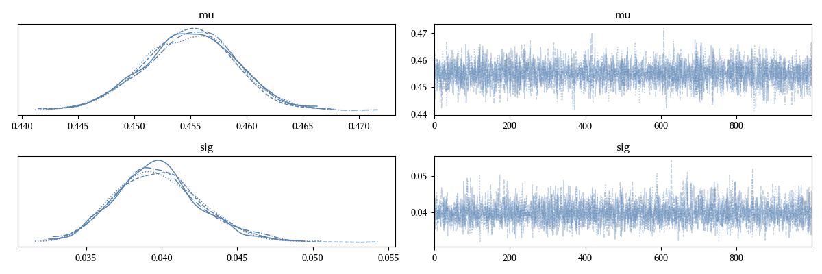
az.plot_trace(trace)
fig = plt.gcf()
fig.tight_layout()

The trace looks fine, as usual.

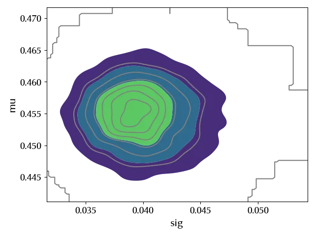
Since we are dealing with two variables, looking at the single marginal distributions only gives us some partial information about the structure of the posterior. We can gain some information by looking at the joint distribution as follows

az.plot_pair(trace, var_names=['sig', 'mu'],
            kind='kde')

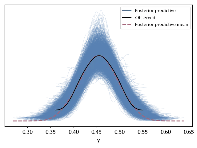
Let us verify our posterior predictive.

with model:
    ppc = pm.sample_posterior_predictive(trace, random_seed=rng)

az.plot_ppc(ppc)

As expected, the agreement is almost perfect.

Conclusions

We showed that dealing with real-valued data requires no modifications to the method discussed in the previous posts. Starting from the next post, we will discuss how to deal with more advanced models.

%load_ext watermark

%watermark -n -u -v -iv -w -p xarray,pytensor

Last updated: Wed Nov 20 2024

Python implementation: CPython
Python version : 3.12.7
IPython version : 8.24.0

xarray : 2024.9.0
pytensor: 2.25.5

arviz : 0.20.0
numpy : 1.26.4
pandas : 2.2.3
matplotlib: 3.9.2
pymc : 5.17.0

Watermark: 2.4.3