Stochastic volatility models

In finance, time series are commonly used to quantify the risk associated with an investment, and many models have been developed for this taks. Here we will show a particular kind of model, named the “stochastic volatility model”. We will use this kind of model to perform a nowcasting, which is the analysis of the current value of a given quantity. Volatility cannot be measured, but we can use SVMs to quantify it. We will use yahoo finance to download the stock value of the largest EU automotive corporations, and we will use PyMC to quantify the associated volatility.

The dataset

Let us first of all download the data. We will use Stellantis, Volks-Wagen, BMW, Mercedes and Renault as study group.

import datetime
import pandas as pd
import numpy as np
import seaborn as sns
import yfinance as yf
import pymc as pm
import arviz as az
from matplotlib import pyplot as plt


tk_names = ['VOW3.DE', 'STLAM.MI', 'BMW.DE', 'MBG.DE', 'RNO.PA']

start_date = datetime.datetime(2024, 1, 1)

end_date = datetime.datetime(2025, 5, 1)

out = {}
for tk_name in tk_names:
    tk = yf.Ticker(tk_name)
    out[tk_name] = np.log(tk.history(start=start_date, end=end_date)['Close'])

df = pd.DataFrame(out).reset_index()

df['Date'] = pd.to_datetime(df['Date'])

# There are few NaNs due to local holidays, we will simply drop them
dfn = df[~df.isna().astype(int).max(axis=1).astype(bool)]

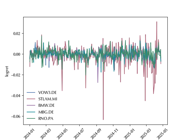
The close value is not appropriate for our inference, and we will use the log-return

out_lr = {}
for tk in tk_names:
    out_lr[tk] = np.diff(np.log(dfn[tk]))

df_lr = pd.DataFrame(out_lr)
df_lr['Date'] = df['Date']

# reordering the columns
df_ord = df_lr[['Date']+list(df_lr.columns[:-1])]

dfr_long = df_ord.melt(id_vars='Date', value_vars=df_ord.columns[1:], value_name='logret', var_name='tk')

fig, ax = plt.subplots()
sns.lineplot(dfr_long, y='logret', x='Date', hue='tk', ax=ax)
legend = ax.legend(frameon=False)
ax.set_xticklabels(ax.get_xticklabels(), rotation=45)

The model

We are now ready to set up our model. In order to build our SVM, we will use a simple gaussian random walk prior for the log-volatility. We recall that a gaussian random walk is the cumulative sum of iid gaussian random variables.

yobs = df_ord['STLAM.MI']*100

with pm.Model() as model:
    lam = pm.Exponential('lam', 0.1)
    rho = pm.GaussianRandomWalk('rho', mu=0, sigma=lam, shape=(len(yobs)))
    sigma = pm.Deterministic('sigma', pm.math.exp(rho/2))
    y = pm.Normal('y', mu=0, sigma=sigma, observed=(yobs - np.mean(yobs)))

rng = np.random.default_rng(42)
kwargs = dict(
    nuts_sampler='numpyro',
    draws=2000,
    tune=2000,
    random_seed=rng
)

with model:
    idata = pm.sample(**kwargs)

az.plot_trace(idata, var_names='lam')
fig = plt.gcf()
fig.tight_layout()

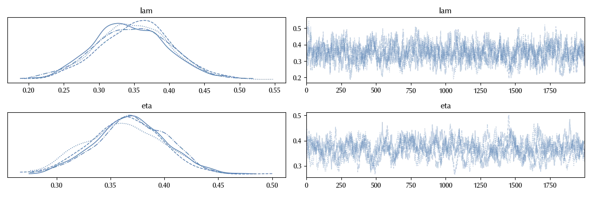
The above trace roughly looks ok (we should increase the number of samples for a proper inference, but it’s ok for our purposes).

We are now ready to inspect our results.

x_ind = df_lr['Date']
t_ind = np.arange(len(x_ind))

fig, ax = plt.subplots(nrows=2, sharex=True)
sns.lineplot(x=t_ind, y=yobs, ax=ax[0])
az.plot_hdi(x=t_ind, y=idata.posterior['sigma'], ax=ax[1])
az.plot_hdi(x=t_ind, y=idata.posterior['sigma'], ax=ax[1], hdi_prob=0.05, color='grey')
xticks = ax[1].get_xticks()
ax[1].set_xticks(xticks[1:8].astype(int))
ax[1].set_xticklabels(x_ind.iloc[xticks[1:8].astype(int)].dt.strftime('%Y-%m-%d'), rotation=45)
ax[1].set_xlim([t_ind[0], t_ind[-1]])
fig.tight_layout()

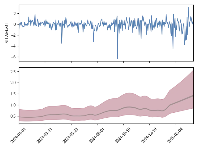
We can see a clear increase in the volatility from January 2025, and if you have ever opened a newspaper in 2025 you might likely guess what’s the cause…

Making the above model hierarchical

We can leverage hierarchical models to quantify families of stocks. As an example, we can assume that the log-volatilities of the above stocks are iid from the log-volatility of the EU automotive market. In this way we gave an implicit operative definition of the log-volatility of the EU automotive market.

yobs_n = df_ord[df_ord.columns[1:]]

coords = {'date': df_ord['Date'],
         'tk': df_ord.columns[1:]}

with pm.Model(coords=coords) as model_h:
    lam = pm.Exponential('lam', 0.1)
    mu_v = pm.GaussianRandomWalk('mu_v', mu=0, sigma=lam, shape=(len(yobs_n )))
    mu = pm.Deterministic('mu', mu_v, dims=('date'))
    eta = pm.HalfNormal('eta', 5)
    rho = pm.Normal('rho', mu=mu[:, None], sigma=eta, dims=('date', 'tk'))
    sigma = pm.Deterministic('sigma', pm.math.exp(rho), dims=('date', 'tk'))
    y = pm.Normal('y', mu=0, sigma=sigma, observed=(yobs_n-yobs_n.mean(axis=0))*100, dims=('date', 'tk'))

with model_h:
    idata_h = pm.sample(**kwargs)

az.plot_trace(idata_h, var_names=['lam', 'eta'])
fig = plt.gcf()
fig.tight_layout()

fig, ax = plt.subplots()
az.plot_hdi(x=t_ind, y=idata_h.posterior['mu'], ax=ax)
az.plot_hdi(x=t_ind, y=idata_h.posterior['mu'], ax=ax, hdi_prob=0.05, color='grey')
xticks = ax.get_xticks()
ax.set_xticks(xticks[1:8].astype(int))
ax.set_xticklabels(x_ind.iloc[xticks[1:8].astype(int)].dt.strftime('%Y-%m-%d'), rotation=45)
ax.set_xlim([t_ind[0], t_ind[-1]])
ax.set_title('EU automotive log volatility')
fig.tight_layout()

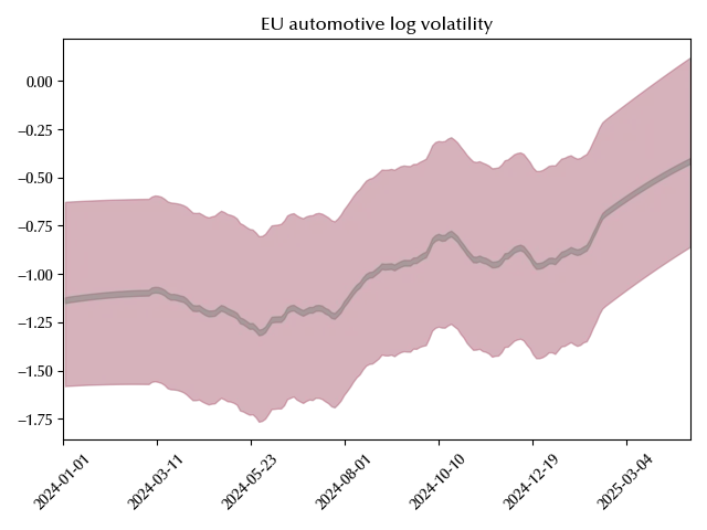
The behavior since January 2025 is analogous to the one previously obtained. Let us now inspect the posterior predictive.

with model_h:
    idata_h.extend(pm.sample_posterior_predictive(idata_h))

fig, ax = plt.subplots(nrows=len(df_ord.columns[1:]), sharex=True, figsize=(6, 6))
for k, col in enumerate(df_ord.columns[1:]):
    sns.lineplot(x=t_ind, y=df_ord[col]*100-df_ord[col].mean(axis=0)*100, ax=ax[k])
    az.plot_hdi(x=df_ord.index, y=idata_h.posterior_predictive['y'].sel(tk=col), ax=ax[k])
xticks = ax[-1].get_xticks()
ax[-1].set_xticks(xticks[1:8].astype(int))
ax[-1].set_xticklabels(df_ord['Date'].iloc[xticks[1:8].astype(int)].dt.strftime('%Y-%m-%d'), rotation=45)
ax[-1].set_xlim([t_ind[0], t_ind[-1]])
fig.tight_layout()

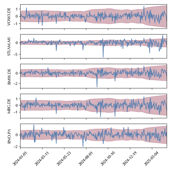
From the above figure, it looks like the increase in the EU automotive volatility is dominated by the large fluctuations of the Stellantis group. To verify this, we could try and fit an SVM model for the remaining stocks, and this is left to the reader.

Conclusions

Time series can be both used to model the time dependence of the mean and to model the time dependence of the variance, and SVM are a popular tool for the latter task.

%load_ext watermark

%watermark -n -u -v -iv -w -p xarray,numpyro

Last updated: Mon May 05 2025

Python implementation: CPython
Python version : 3.12.8
IPython version : 8.31.0

xarray : 2025.1.1
numpyro: 0.16.1

pymc : 5.22.0
pandas : 2.2.3
numpy : 2.2.5
arviz : 0.21.0
matplotlib: 3.10.1
yfinance : 0.2.54
seaborn : 0.13.2

Watermark: 2.5.0