Structural time series

In the last post we allowed for autocorrelation across measures. In this post we will adapt our model to include other forms of temporal dependencies. We will use the dataset used by Harvey and Durbin in the well known 1986 study on the british seat belt legislation. The raw data can be found in this repo.

The study analyzes the impact of the 1983 seat belt legislation which made seat belts mandatory on the monthly number of deceased or seriously injured car drivers.

import pandas as pd
import seaborn as sns
import pymc as pm
import arviz as az
import numpy as np
from matplotlib import pyplot as plt
import pytensor as pt

rng = np.random.default_rng(42)

df = pd.read_csv('https://raw.githubusercontent.com/thestippe/thestippe.github.io/main/data/seatbelt_uk_harvey.csv')

df['Date'] = pd.to_datetime(df['Date'])

fig = plt.figure()
ax = fig.add_subplot(111)
sns.lineplot(df, x='Date', y='drivers', ax=ax)
ax.axvline(x=df[df['law']==1]['Date'].min(), ls=':', color='grey')

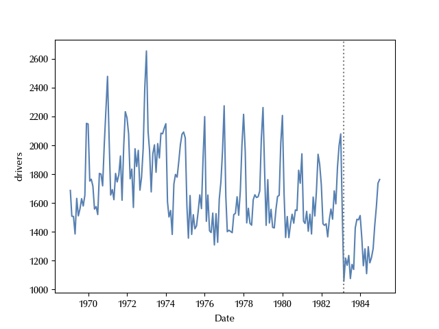
The data shows a strong periodic (yearly) component, and this seems quite reasonable, due to bad road conditions in winter caused by ice and other climate-related factors.

df['month'] = df['Date'].dt.month
sns.barplot(df.groupby('month').mean()['drivers'].reset_index(), y='drivers', x='month')

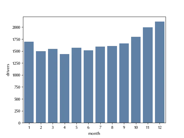
We can add a periodic component by expanding it into its Fourier series

\[f(t) = \sum_{j=1}^\infty \left( a_j \cos(\omega_j t) + b_j \sin(\omega_j t) \right)\]

where $\omega_j = \frac{2 \pi j}{T}\,,$ and $T$ is the period, which is assumed to be 12 months (1 year). What one usually expects is that high frequency components becomes less and less important as the frequency increases. Moreover, those components are generally hidden by statistical noise. Therefore, only the first few components are considered as relevant. We will only include the $j=1,2$ component, but you are encouraged to test what happens when we also include higher frequencies such as $j=3\,.$

Since we want to assess the effect of the law introduction, we will also include it as a regressor. As the author, we will include two other regressors:

The total number of kilometers travelled by cars in one month
The real petrol price.

x = np.arange(0, len(df)/12, 1/12)
T = 12

with pm.Model() as model_start:
    tau = pm.Exponential('tau', 0.1)
    rho = pm.Normal('rho', mu=0, sigma=2, shape=(2))
    gamma = pm.Normal('gamma', mu=0, sigma=2, shape=(3))
    alpha = pm.AR('alpha', rho=rho, tau=tau, shape=len(df['drivers']))
    beta = pm.Normal('beta', 0, 2, shape=(2, 2))
    mu = pm.Deterministic('mu', alpha
                          +beta[0][0]*pm.math.cos(2.0*np.pi*x)+beta[0][1]*pm.math.sin(2.0*np.pi*x)
                          +beta[1][0]*pm.math.cos(4.0*np.pi*x)+beta[1][1]*pm.math.sin(4.0*np.pi*x)
                          + gamma[0]*df['law'] + gamma[2]*df['kms']/10000 + gamma[1]*df['PetrolPrice']*10 
                         )
    sigma = pm.HalfNormal('sigma', 1)
    y = pm.Normal('y', mu=mu, sigma=sigma, observed=df['drivers']/1000)
    idata_start = pm.sample(nuts_sampler='numpyro', draws=80000, tune=80000,
                            target_accept=0.8, random_seed=rng)

az.plot_trace(idata_start, var_names=['rho', 'tau', 'sigma', 'beta', 'gamma'])
fig = plt.gcf()
fig.tight_layout()

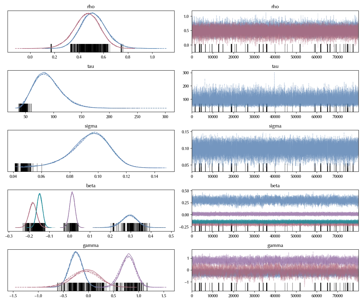
The trace shows some minor issue despite the large number of samples. Let us take a look at the trace summary:

az.summary(idata_start, var_names=['rho', 'tau', 'sigma', 'beta', 'gamma'])

	mean	sd	hdi_3%	hdi_97%	mcse_mean	mcse_sd	ess_bulk	ess_tail	r_hat
rho[0]	0.519	0.106	0.322	0.721	0.001	0.001	13654	20562	1
rho[1]	0.463	0.107	0.258	0.661	0.001	0.001	12274	20504	1
tau	90.382	24.43	47.543	135.72	0.322	0.228	5004	6822	1
sigma	0.094	0.014	0.066	0.12	0	0	5372	4507	1
beta[0, 0]	0.294	0.038	0.221	0.366	0.001	0.001	1059	2378	1
beta[0, 1]	-0.181	0.019	-0.216	-0.145	0	0	19573	34387	1
beta[1, 0]	0.013	0.013	-0.012	0.038	0	0	22893	42960	1
beta[1, 1]	-0.147	0.014	-0.173	-0.122	0	0	11107	35174	1
gamma[0]	-0.248	0.13	-0.493	-0.002	0.001	0.001	9738	17987	1
gamma[1]	-0.063	0.27	-0.57	0.438	0.012	0.008	550	1176	1
gamma[2]	0.786	0.147	0.506	1.056	0.005	0.003	913	1953	1

Let us now compare the posterior predictive distribution with the observed data.

with model_start:
    idata_start.extend(pm.sample_posterior_predictive(idata_start))

fig = plt.figure()
ax = fig.add_subplot(111)
ax.fill_between(df['Date'], 1000*idata_start.posterior_predictive['y'].quantile(q=0.03, dim=('draw', 'chain')),
               1000*idata_start.posterior_predictive['y'].quantile(q=0.97, dim=('draw', 'chain')),
               color='lightgray', alpha=0.8)
ax.plot(df['Date'], 1000*idata_start.posterior_predictive['y'].mean(dim=('draw', 'chain')))
ax.axvline(x=df[df['law']==1]['Date'].min(), color='k', ls=':')
sns.lineplot(df,x='Date', y='drivers', ax=ax)

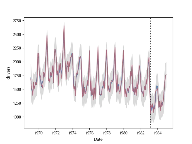
We can perfectly account for most of the data, so our model seems capable to almost perfectly reproduce all the relevant features. Notice that $\gamma_0$ is well below 0, so there are no doubts that, according to our model, the law introduction had a positive impact on the driver safety. On average, the seat belt introduction reduced by 250 the number of seriously injured drivers.

Conclusions

We have seen how to include external dependencies such as periodic or trend components as well as autoregressive patterns in a time series regression by using structural time series.

Conclusions

Suggested readings