Time series

While many models assume independence of the observations, here we will start to see how to include temporal dependence into our models. There are many kinds of temporal dependence:

short term correlation
seasonality
trends
…

As an example, let us try and assume we are trying to model the temporal dependence of the daily temperature for a certain location. We assume that the observed temperature at a given day $t$ is given by

$y_t = \mu_t + \varepsilon_t$

where $\varepsilon_t$ is a zero-mean error term. Today’s daily average temperature of the location is probably closer to yesterday’s daily average temperature of the same location then to the one of one week ago, so we might assume that there is short term correlation. Moreover, today’s average temperature is probably closer to the average temperature registered one year ago than to the one of six months ago, we should therefore incorporate seasonality into our model. Finally, if your data goes over many years, you might also want to include a trend term into our model in order to account for the observed trend in the average global temperature.

In this post, we will see how to include short term correlation by using Auto-Regressive (AR) models, while in the next post we will discuss how to include other kinds of temporal dependencies.

As a remark, it is important to distinguish between time series, where one usually wants to model the temporal dependence of one/few individuals, and longitudinal models, where the aim is to describe the evolution of a population made up by many individuals over time. Longitudinal models have already been introduced in this post about random models, and will be discussed more in depth into a future post.

The autoregressive model

Let us assume that we are trying and model the temporal dependence of a model as the one above

$y_t = \mu_t + \varepsilon_t\,.$ where $t=1,2,\dots,T\,.$

If we assume that the expected daily temperature follows an autoregressive model of order $p$, indicated as $AR(p)\,,$ we are saying

\[\mu_t \vert \rho, \sigma, \mu_0 = \rho_0 + \sum_{i=1}^p \rho_i \mu_{t-i} + \eta_t\]

where

\[\eta_t \sim \mathcal{N}(0, \sigma)\,.\]

We also included the dependence on $\mu_0\,,$ since we must also specify it.

Box and Jenkins’ chemical process dataset.

We will analyze the series of 70 consecutive yields from a batch chemical process, from “Time series analysis, forecasting and control”, by Box et al.:

	1	2	3	4	5	6	7	8	9	10	11	12	13	14	15
1	47	64	23	71	38	64	55	41	59	48	71	35	57	40	58
16	64	80	55	37	74	51	57	50	60	45	57	50	45	25	59
31	70	71	56	74	50	58	45	54	36	54	48	55	45	57	50
46	82	44	64	43	52	38	59	55	41	53	49	34	35	54	45
51	88	38	50	60	39	59	40	57	54	23

import pandas as pd
import seaborn as sns
import pymc as pm
import arviz as az
import numpy as np
from scipy.stats import norm
from matplotlib import pyplot as plt

rng = np.random.default_rng(42)

n_draws = 2000
n_chains = 4

df_tmp = pd.read_csv('https://www.stat.purdue.edu/~chong/stat520/bjr-data/chem-yields',
                     header=None, sep=' ')

df_tmp = df_tmp.drop(columns=[0])

vals = np.concatenate([df_tmp.iloc[n].dropna().values for n in df_tmp.index])

df = pd.DataFrame({'x': np.arange(len(vals)), 'y': vals})

sns.lineplot(df, x='x', y='y')c

The yield of the chemical process

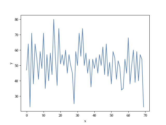
What happens here is that high-yielding batches produce residuals which are not remove from the vessel. Due to these residuals, the subsequent batch tend to be a low-yield one. There is a clear autoregressive pattern, while there is no clear periodic or trend component, and we will therefore assume a purely autoregressive model. We will not fit the last 5 points in order to use them to assess the predictive power of the model. In order to keep the model variables of order 1, we will divide the yield by 100.

df['y_fit'] = df['y']/100

n_fit = len(df)-5

df_fit = df.iloc[:n_fit]
df_pred = df.iloc[n_fit:]

yfit = df_fit['y_fit']
ypred = df_pred['y_fit']

with pm.Model() as model_1:
    tau = pm.Exponential('tau', 0.01)
    rho = pm.Normal('rho', mu=0, sigma=2, shape=(2))
    mu = pm.AR('mu', rho=rho, tau=tau, ar_order=2, shape=len(yfit))
    sigma = pm.HalfNormal('sigma', 5)
    y = pm.Normal('y', mu=mu, sigma=sigma, observed=(yfit))

with model_1:
    idata_1 =  pm.sample(nuts_sampler='numpyro', draws=n_draws, tune=n_draws, chains=n_chains,
                         target_accept=0.95, random_seed=rng)

az.plot_trace(idata_1)
fig = plt.gcf()
fig.tight_layout()

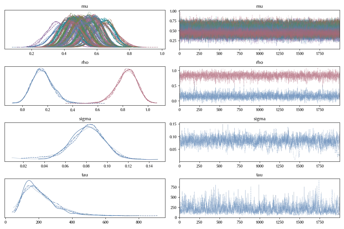
The trace seems ok. Let us now compute the posterior predictive.

with model_1:
    idata_1.extend(pm.sample_posterior_predictive(idata_1, random_seed=rng))

fig = plt.figure()
ax = fig.add_subplot(111)
ax.fill_between(df['x'].iloc[:n_fit],idata_1.posterior_predictive['y'].quantile(q=0.03, dim=('draw', 'chain')),
                idata_1.posterior_predictive['y'].quantile(q=0.97, dim=('draw', 'chain')),
               color='lightgray', alpha=0.8)
ax.plot(df['x'].iloc[:n_fit],  idata_1.posterior_predictive['y'].mean(dim=('draw', 'chain')))
sns.lineplot(df,x='x', y='y_fit', ax=ax)

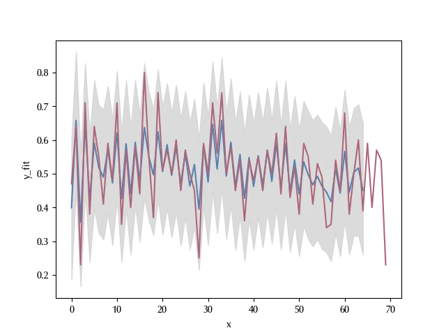
The expected average closely resembles the observed data, so our model seems quite appropriate. Let us now verify the predictive power of the model.

with model_1:
    pm.compute_log_likelihood(idata_1)

with model_1:
    mu_pred = pm.AR('mu_pred', rho=rho, tau=tau, ar_order=2,
                    init_dist=pm.DiracDelta.dist(mu[...,-1]), shape=len(df.iloc[n_fit-1:]))
    y_pred = pm.Normal('y_pred', mu=mu_pred[1:], sigma=sigma)

with model_1:
    ppc_1 = pm.sample_posterior_predictive(idata_1, var_names=['mu_pred', 'y_pred'])

idt_1 = np.concatenate([idata_1.posterior_predictive['y'].values.reshape((n_draws*n_chains, -1)),
                        ppc_1.posterior_predictive['y_pred'].values.reshape((n_draws*n_chains, -1))], axis=(1))

fig = plt.figure()
ax = fig.add_subplot(111)
ax.fill_between(df['x'], np.quantile(idt_1, q=0.03, axis=0),
                np.quantile(idt_1, q=0.97, axis=0),
               color='lightgray', alpha=0.8)
ax.plot(df['x'],  idt_1.mean(axis=0))
ax.axvline(x=df['x'].iloc[n_fit], ls=':', color='grey')
ax.set_ylim([0, 1])
sns.lineplot(df,x='x', y='y_fit', ax=ax)

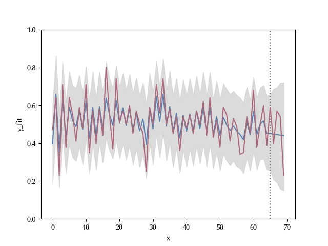
The forecasted series does not show the previous pattern, and this might be a limit of our model. Let us verify that a higher order autoregressive model is able to encode this feature.

with pm.Model() as model_2:
    tau = pm.Exponential('tau', 0.01)
    rho = pm.Normal('rho', mu=0, sigma=2, shape=(3))
    mu = pm.AR('mu', rho=rho, tau=tau, ar_order=3, shape=len(yfit))
    sigma = pm.HalfNormal('sigma', 5)
    y = pm.Normal('y', mu=mu, sigma=sigma, observed=(yfit))

with model_2:
    idata_2 =  pm.sample(nuts_sampler='numpyro', draws=n_draws, tune=n_draws, chains=n_chains,
                         target_accept=0.95, random_seed=rng)

az.plot_trace(idata_2)
fig = plt.gcf()
fig.tight_layout()

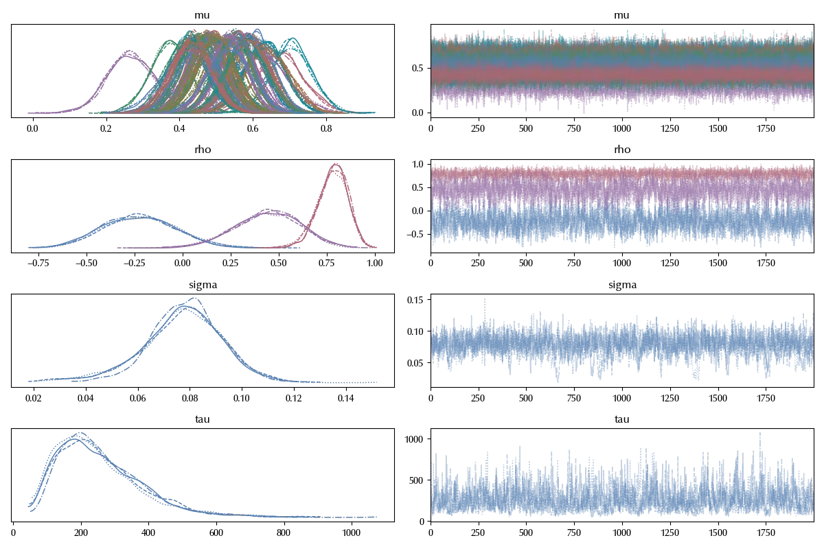
Also in this case the trace is fine. Let us check if our model is able to correctly forecast the first few observations.

with model_2:
    idata_2.extend(pm.sample_posterior_predictive(idata_2, random_seed=rng))

with model_2:
    mu_pred = pm.AR('mu_pred', rho=rho, tau=tau, ar_order=3, 
                    init_dist=pm.DiracDelta.dist(mu[...,-2], mu[...,-1], shape=(2)),
                    shape=(2+len(df_pred)))
    y_pred = pm.Normal('y_pred', mu=mu_pred[2:], sigma=sigma)

with model_2:
    ppc_2 = pm.sample_posterior_predictive(idata_2, var_names=['mu_pred', 'y_pred'])

idt_2 = np.concatenate([idata_2.posterior_predictive['y'].values.reshape((n_draws*n_chains, -1)),
                        ppc_2.posterior_predictive['y_pred'].values.reshape((n_draws*n_chains, -1))], axis=(1))

fig = plt.figure()
ax = fig.add_subplot(111)
ax.fill_between(df['x'], np.quantile(idt_2, q=0.03, axis=0),
                np.quantile(idt_2, q=0.97, axis=0),
               color='lightgray', alpha=0.8)
ax.plot(df['x'],  idt_2.mean(axis=0))
ax.axvline(x=df['x'].iloc[n_fit], ls=':', color='grey')
ax.set_ylim([0, 1])
sns.lineplot(df,x='x', y='y_fit', ax=ax)

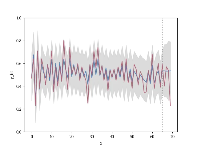
The model seems to correctly reproduce the one-step-ahead distribution, but then it shows the same issue of the $AR(1)$ model.

Conclusions

We have seen how to implement an autoregressive model in PyMC and how to assess its forecasting performances. In the next post, we will discuss how to include external time dependencies such as trend or periodic patterns

	1	2	3	4	5	6	7	8	9	10	11	12	13	14	15
1	47	64	23	71	38	64	55	41	59	48	71	35	57	40	58
16	64	80	55	37	74	51	57	50	60	45	57	50	45	25	59
31	70	71	56	74	50	58	45	54	36	54	48	55	45	57	50
46	82	44	64	43	52	38	59	55	41	53	49	34	35	54	45
51	88	38	50	60	39	59	40	57	54	23

	1	2	3	4	5	6	7	8	9	10	11	12	13	14	15
1	47	64	23	71	38	64	55	41	59	48	71	35	57	40	58
16	64	80	55	37	74	51	57	50	60	45	57	50	45	25	59
31	70	71	56	74	50	58	45	54	36	54	48	55	45	57	50
46	82	44	64	43	52	38	59	55	41	53	49	34	35	54	45
51	88	38	50	60	39	59	40	57	54	23

The autoregressive model

Box and Jenkins’ chemical process dataset.

Conclusions

Suggested readings

	1	2	3	4	5	6	7	8	9	10	11	12	13	14	15
1	47	64	23	71	38	64	55	41	59	48	71	35	57	40	58
16	64	80	55	37	74	51	57	50	60	45	57	50	45	25	59
31	70	71	56	74	50	58	45	54	36	54	48	55	45	57	50
46	82	44	64	43	52	38	59	55	41	53	49	34	35	54	45
51	88	38	50	60	39	59	40	57	54	23