Quantile regression

In the last post we discussed the GEV distribution as well as the generalized Pareto distribution, which are two distributions emerging from extreme value theory, one of the main approaches to tail analysis. In this post, we will introduce another relevant approach in the context of tail analysis, namely the quantile regression.

The aim of quantile regression is to determine the dependence of a given quantile $q$ of the data on one or more regressors. As an example, if your aim is to study underweight babies, then ordinary regression is not a suitable tool, and quantile regression can be a smart choice in this context.

Quantile regression can be also used in the context of classification, when you want to find out values which are too extreme (higher than the $p$-th quantile), you can first perform a quantile regression and then compare the new observations with the value for the expected $p$-th quantile.

In Bayesian statistics, quantile regression can be implemented by using the asymmetric Laplace distribution, which can be parametrized in terms of a quantile parameter $q$.

Example

In our example we will use the dataset provided in this blog

We will consider three columns:

bwt the birth weight of the baby
age the age of the mother
smoke 1 if the mother smokes, 0 otherwise

import pandas as pd
import numpy as np
import seaborn as sns
import pymc as pm
import arviz as az
from matplotlib import pyplot as plt

df = pd.read_csv('http://people.hsc.edu/faculty-staff/blins/classes/spring17/math222/data/babies.csv')

df.head()

	case	bwt	gestation	age	height	weight	smoke
0	1	120	284	27	62	100	0
1	2	113	282	33	64	135	0
2	3	128	279	28	64	115	1
4	5	108	282	23	67	125	1
5	6	136	286	25	62	93	0

The dataset contains few null value, and we will simply drop them

df = df.dropna()
sns.histplot(df, x='bwt')

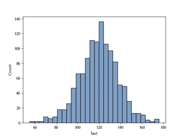
We will try and determine the first, second and third quartiles of the birth weight depending on the age and on the smoke field.

yobs = df['bwt'].values/100
quantiles = np.array([0.25, 0.5, 0.75])

coords = {'q': np.arange(len(quantiles)),
         'obs': np.arange(len(yobs))}

ystack = np.array([yobs]*np.shape(quantiles)[0])

X = np.array(df['age'].values).reshape((1, -1))
smoke = np.array(df['smoke'].values).reshape((1, -1))

with pm.Model(coords=coords) as model:
    alpha = pm.Normal('alpha', mu=0, sigma=10, dims=('q'))
    beta = pm.Normal('beta', mu=0, sigma=2, dims=('q'))
    gamma = pm.Normal('gamma', mu=0, sigma=2, dims=('q'))
    sigma = pm.HalfNormal('sigma', 20)
    eta = pm.Deterministic('eta', alpha + beta*X.T, dims=('obs', 'q'))
    phi = pm.Deterministic('phi', alpha + beta*X.T + gamma, dims=('obs', 'q'))
    mu = pm.Deterministic('mu', alpha + beta*X.T + gamma*smoke.T, dims=('obs', 'q'))
    y = pm.AsymmetricLaplace('y', q=quantiles.T, mu=mu, b=sigma, observed=ystack.T)

rng = np.random.default_rng(42)

kwargs = dict(chains=4,
             draws=2000,
             tune=2000,
             random_seed=rng,
             nuts_sampler='numpyro')

$\phi$ and $\eta$ will be simply used in the posterior predictive check, while $\mu$ actually represents the expected value for the $q$-th quantile.

pm.model_to_graphviz(model)

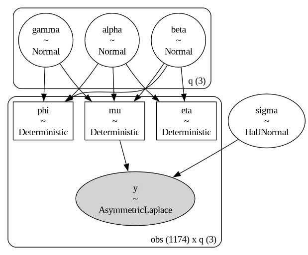
In our model, we have a distinct set of regressors ($\alpha$, $\beta$ and $\gamma$) for each quantile value, while we assume a single value for $\sigma$.

rng = np.random.default_rng(42)

kwargs = dict(chains=4,
             draws=2000,
             tune=2000,
             random_seed=rng,
             nuts_sampler='numpyro')

with model:
    idata = pm.sample(**kwargs)
    
az.plot_trace(idata, var_names=['alpha', 'beta', 'gamma','sigma'])
fig = plt.gcf()
fig.tight_layout()

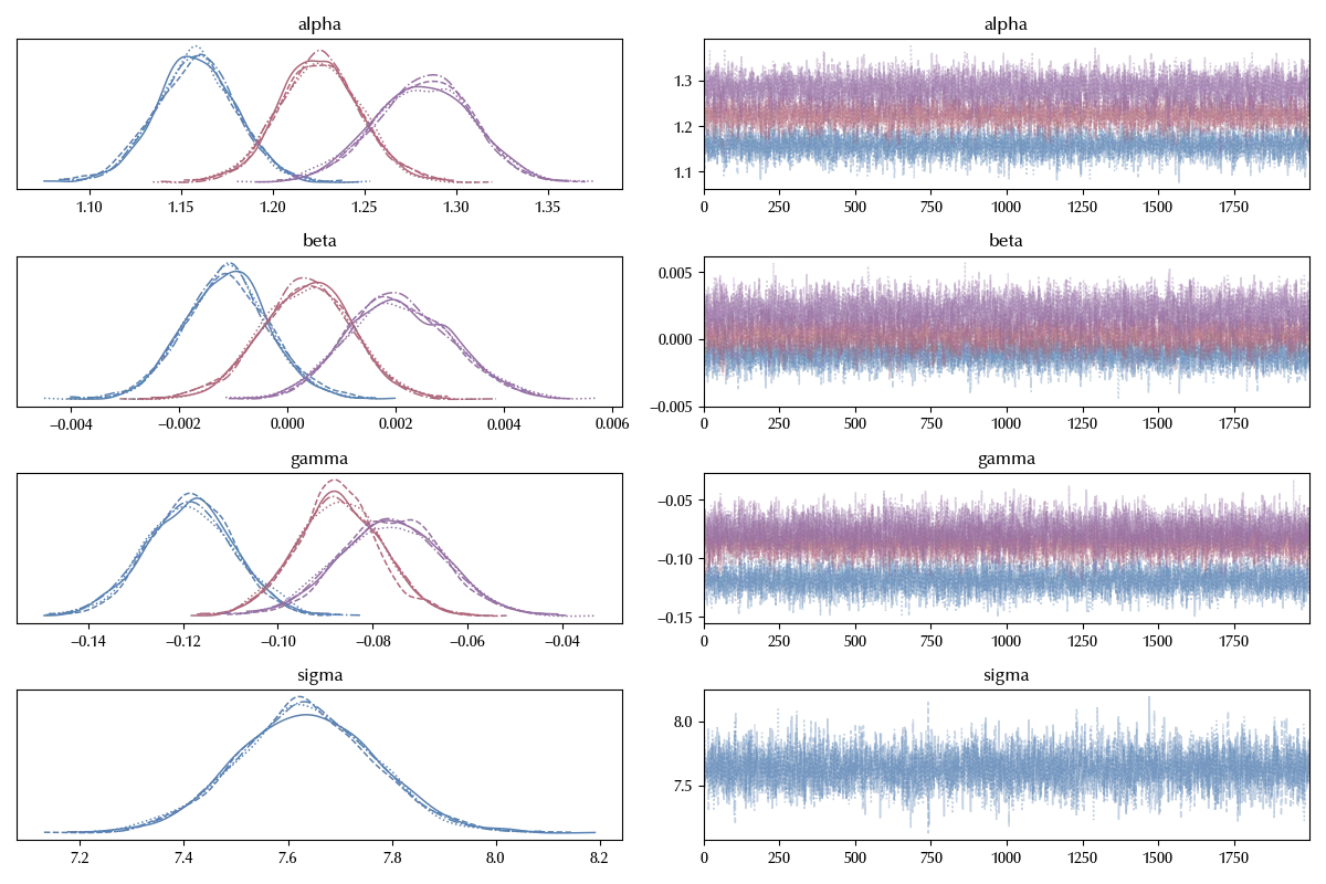
The trace looks OK, let us inspect our estimate for the quantiles.

fig, ax = plt.subplots()
for k, q in enumerate(quantiles):
    ax.plot(X.reshape(-1), idata.posterior['eta'].sel(q=k).mean(dim=('draw', 'chain')),
           color=f'C{k}', label=f"Non-smoker q={str(q)}")
for k, q in enumerate(quantiles):
    ax.plot(X.reshape(-1), idata.posterior['phi'].sel(q=k).mean(dim=('draw', 'chain')),
           color=f'C{k}', ls=':', label=f"Smoker q={str(q)}")
ax.scatter(X.reshape(-1), yobs, marker='x', color='lightgray')
legend = ax.legend(bbox_to_anchor=(0.99, 1.0), frameon=False)

The posterior predictive plot

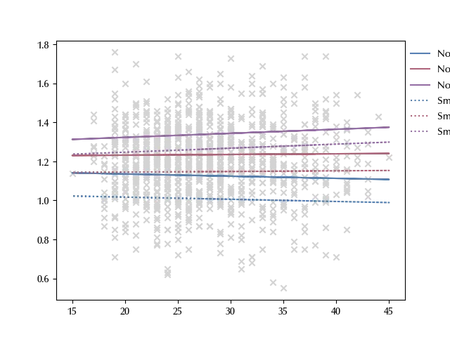
As we can see, the median weight value for babies with smoking mother is compatible with the first quartile weight value of the babies with non-smoking mother.

Conclusions

Quantile regression can be a valid tool if your aim is to make inference on rare situations, and it can be easily implemented with PyMC.

	case	bwt	gestation	age	height	weight	smoke
0	1	120	284	27	62	100	0
1	2	113	282	33	64	135	0
2	3	128	279	28	64	115	1
4	5	108	282	23	67	125	1
5	6	136	286	25	62	93	0

	case	bwt	gestation	age	height	weight	smoke
0	1	120	284	27	62	100	0
1	2	113	282	33	64	135	0
2	3	128	279	28	64	115	1
4	5	108	282	23	67	125	1
5	6	136	286	25	62	93	0

Example

Conclusions

Suggested readings

	case	bwt	gestation	age	height	weight	smoke
0	1	120	284	27	62	100	0
1	2	113	282	33	64	135	0
2	3	128	279	28	64	115	1
4	5	108	282	23	67	125	1
5	6	136	286	25	62	93	0