Introduction to Extreme Values theory

In some circumstances you may be not interested in modelling the distribution itself, but you may be interested in understanding its asymptotic behavior, and the extreme value theory is the discipline which studies this topic.

Extreme value theory is unique as a statistical discipline in that it develops techniques and models for describing the unusual rather than the usual.

Stuart Coles

The EV theory is appropriate when you want to investigate the distribution of the minimum or maximum value of some quantity, as the maximum loss of a financial asset or the yearly maximum volume of rain in a certain location.

The intuition behind the extreme value theory is that any probability distribution function is positive and must integrate to one, it must therefore fall to zero fast enough if $x \rightarrow \infty\,.$ This puts strong constraints to its asymptotic behavior, and this leads to the Fisher-Tippet-Gnedenko theorem.

Formally if we have a continuous positive random variable $X$ with cumulative distribution function $F(x)\,,$ and we observe $X_1,…,X_n$ independent identically distributed variables distributed according to $X\,,$ if we denote $M_n$ the maximum of $X_1,…,X_n\,,$ then

$P(M_n \leq x) = P(X_1 \leq x) P(X_2 \leq x) … P(X_n \leq x) = (F(x))^n\,.$

However, one may not know $F$ a priori, but the FTG theorem states that, if there exist $a_n, b_n \in \mathbb{R}$ such that

\[P\left( \frac{M_n - a_n}{b_n} \leq x \right) \rightarrow G(x)\]

then $G(x) \propto \exp{\left(-(1+ \xi x)^{-1/\xi}\right)}\,.$

Once properly normalized and promoted to a location-scale family one arrives to the Generalized Extreme Value distribution:

\[p(x) = \frac{1}{\sigma} t(x)^{\xi + 1}e^{- t(x)}\]

where

\[t(x) = \begin{cases} \left(1+ \xi \left(\frac{x-\mu}{\sigma}\right)\right)^{-1/\xi}\,& if\,& \xi \neq 0 \\ e^{-\left(x-\mu\right)/\sigma}\,& if\,& \xi = 0\\ \end{cases}\]

Notice that, if $X_1,…, X_n$ are distributed according to $G\,,$ then $\max(X_1,…,X_n)$ is distributed according to $G\,.$ This distribution is known as the Generalized Extreme Value (GEV) distribution.

Maximum distribution of the Apple stocks

I have been working on financial risk assessment for a while, and one of the central issues in this field is to determine the risk due to extremely large fluctuations of the stock market. EVT can be really helpful in this task, and we will show how in this post. We will use Yahoo Finance to download the values of the Apple stock in the period from the January 1st 2020 to the December 31st 2023.

The Generalized Extreme Values distribution is not directly available in PyMC, but can be found in the pymc_experimental package.

import numpy as np
import pandas as pd
import pymc as pm
import pymc_experimental.distributions as pmx
import arviz as az
from matplotlib import pyplot as plt
import yfinance as yf

rng = np.random.default_rng(9876556789)

df = yf.download('AAPL', start='2020-01-01', end='2023-12-01').reset_index()
df['Date'] = pd.to_datetime(df['Date'])
df['LogRet'] = np.log(df['Close']).diff()
df = df.dropna()

First of all, we converted the close values (the value of the stock at the end of the day) into logarithmic-returns (log-returns for short). This is a common operation in finance, since for compound interest assets the total value is

\[\prod_i (1+r_i)\]

If we take the logarithm of the above formula we transform the product into a sum, and this makes log-returns so useful.

We are interested in finding the distribution of the weekly minima of the daily close.

data = df.groupby([pd.Grouper(key='Date', freq='W')])['LogRet'].min().reset_index()
dt = -data['LogRet'].values

Before fitting the model, let us take a look at the behavior of the data

fig = plt.figure()
ax = fig.add_subplot(211)
ax1 = fig.add_subplot(212)

ax.plot(data['Date'], data['LogRet'])
ax1.hist(data['LogRet'], bins=50)
fig.tight_layout()

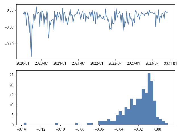
There is some evident time dependence. As an example, we can observe quite a high volatility during the Covid pandemic and another high volatility period after the Ukraine invasion. However, for the moment, we will neglect the time dependence, and assume that the parameters are stationary.

Since we have quite a large amount of data, we can safely use uninformative priors. We do expect that both $\mu$ and $\sigma$ are typically much smaller than one, so we will take a standard deviation of 2 for the first one and equal to 1 for the latter.

From the Wikipedia page we observe that, if $| \xi|>1\,,$ the mean does not exist. Since it is reasonable to assume that it exists, we expect that $\xi$ will be bounded into the $[-1, 1]$ region, therefore we have the following model

with pm.Model() as model_gev:
    mu = pm.Normal('mu', sigma=0.2)
    sigma = pm.HalfNormal('sigma', sigma=0.2)
    xi = pm.Normal('xi', sigma=1)
    gev = pmx.GenExtreme('gev',mu=mu, sigma=sigma, xi=xi, observed=dt)
    trace = pm.sample(tune=2000, draws=2000, chains=4, 
                      nuts_sampler='numpyro', random_seed=rng)

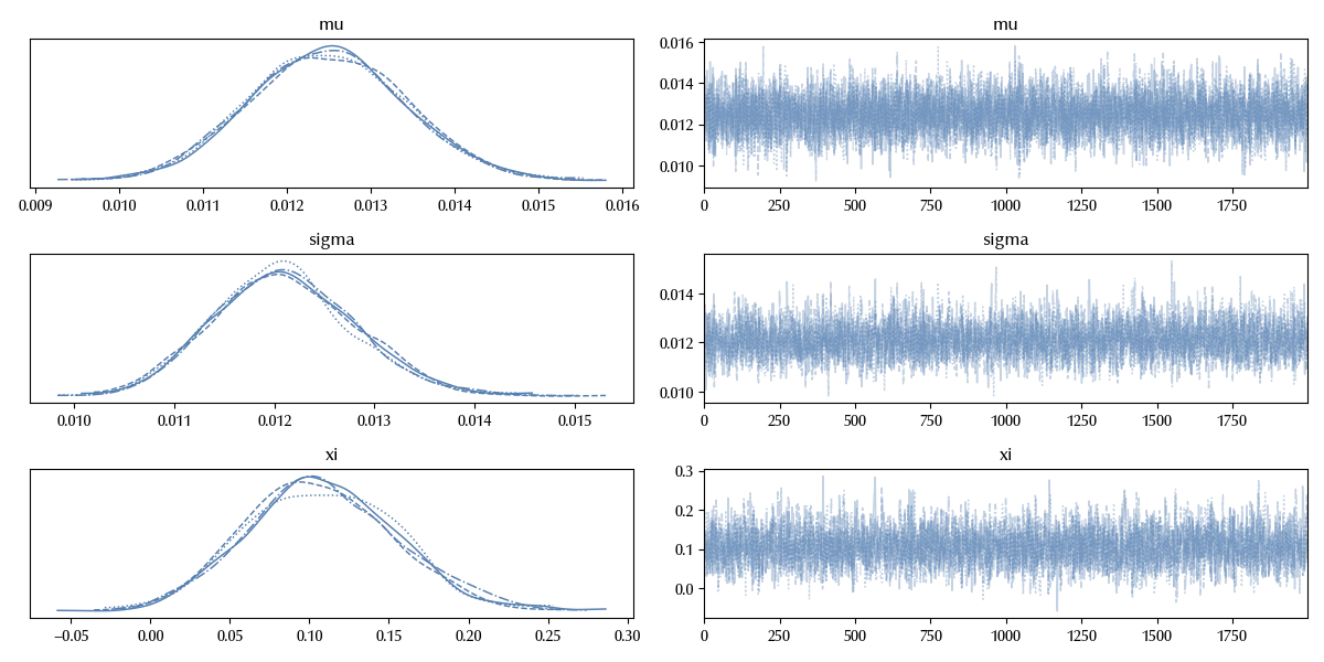
az.plot_trace(trace)

The trace of our model

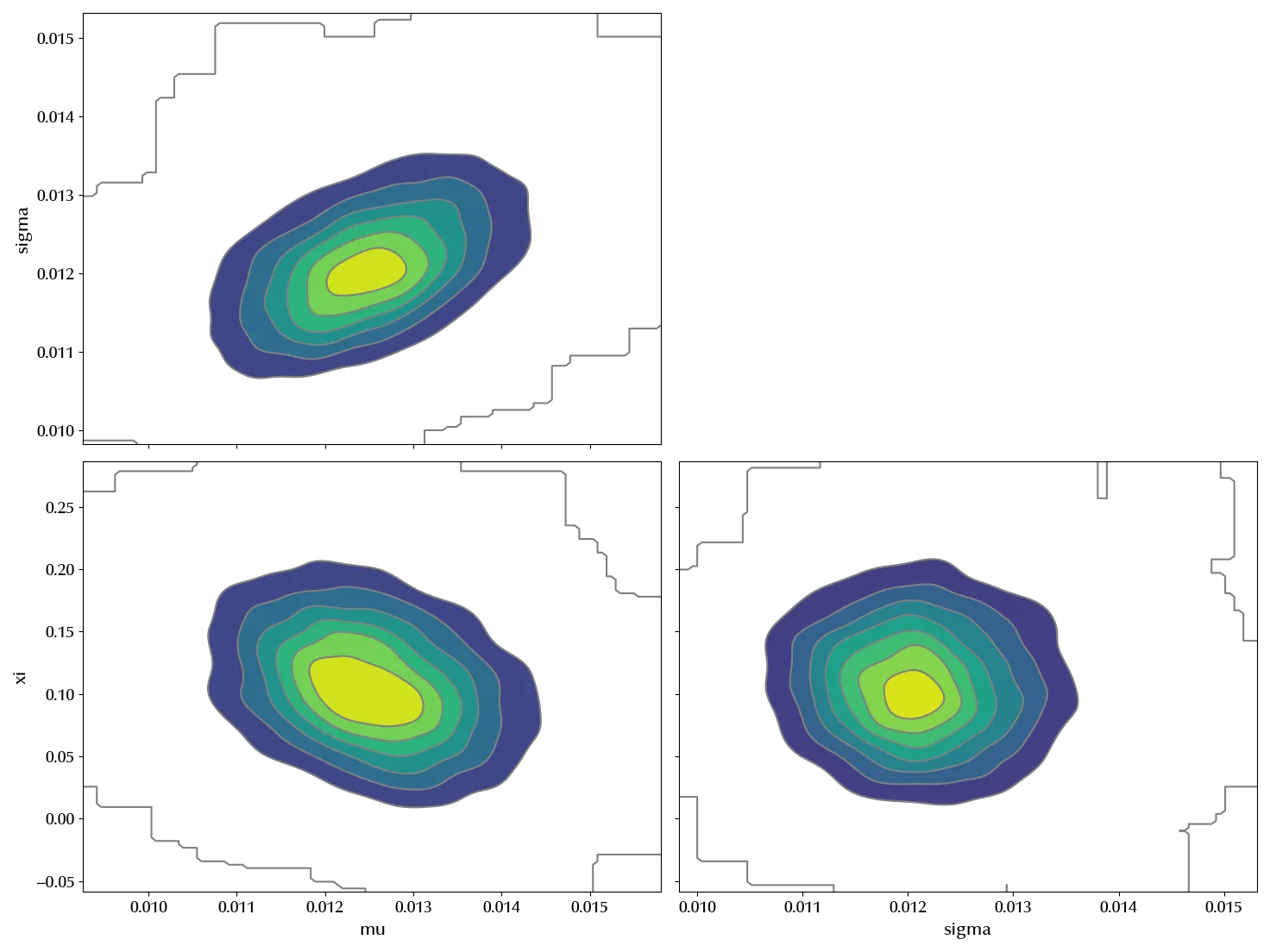
Let us take a look at the joint posterior distribution.

az.plot_pair(trace, kind='kde')
fig = plt.gcf()
fig.tight_layout()

The KDE plot of the posterior distribution

We can now take a look at the PPC in order to verify if our model is able to reproduce the data

with model_gev:
    ppc = pm.sample_posterior_predictive(trace, random_seed=rng)

fig = plt.figure()
ax = fig.add_subplot(111)
az.plot_ppc(ppc, ax=ax, alpha=0.8, kind='kde', num_pp_samples=500)

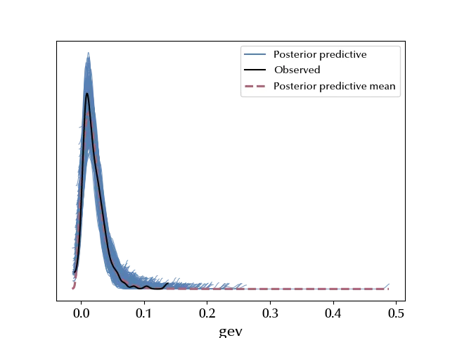
The posterior predictive distribution

There’s a very good agreement between the observed and the predicted values, so our estimate should be quite reliable.

The Generalized Pareto distribution

Keeping only the extreme values may be a waste of information. As an example, we only kept the weekly maxima, so we trowed away four days out of five. In some situation, instead of analyzing what is the distribution probability for the maxima, it may be better to analyze what is the probability that your random variable exceeds some threshold. More precisely, given $u,y>0\,,$ we want to get information on

\[P(X>u+y | X>u) = \frac{P((X>u+y)\cap (X>u))}{P(X>u)} = \frac{P(X>u+y)}{P(X>u)} = \frac{1-F(u+y)}{1-F(u)}\]

It can be proved (see Coles’ textbook for the outline) that, for large enough $u\,,$ the above distribution must have the form

\[p(y | u, \sigma, \xi) = \left(1+\frac{\xi y}{\sigma}\right)^{-1/\xi}\]

The distribution

\[p(y | \mu, \sigma, \xi) = \left(1+\xi \frac{y-\mu}{\sigma}\right)^{-1/\xi}\]

is named the Generalized Pareto Distribution (GPD). For the mathematical details on the above distribution, see the corresponding Wikipedia page.

Now it comes one bad news and one good news. The bad one is that in PyMC it is only implemented the Pareto type I distribution, which is a special case of the GPD. The good one is that it is really easy to implement custom distributions in PyMC, and this can be done following this very nice tutorial. You can find my own implementation on my GitHub repo.

Let us see how to model the tail of the Apple stocks by using it. A reasonably high enough threshold for the log returns is $0.03\,,$ as this value is high enough to be far from the center and low enough to provide a discrete amount of data. We do expect $\sigma \ll 1\,,$ therefore assuming a variance of 1 for it may be enough. $\xi$ must be lower than 1. If it is 1, then the mean does not exist, and this doesn’t make much sense. If $\xi$ is negative, then the support of the GDP has an upper bound, and it doesn’t make much sense too, so we can assume it is non-negative. We can therefore take a half normal distribution for it, with variance 10.

from gen_pareto.generalized_pareto import GPD

thr = 0.03

dt1 = -df[-df['LogRet']>thr]['LogRet'].values

with pm.Model() as pareto_model:
    sigma = pm.HalfNormal('sigma',sigma=1)
    xi = pm.HalfNormal('xi', sigma=10)
    y = GPD('y', mu=thr, sigma=sigma, xi=xi, observed=dt1)
    trace_pareto = pm.sample(draws=2000, tune=2000, chains=4, random_seed=rng,
                            nuts_sampler='numpyro')

az.plot_trace(trace_pareto)

The trace of the Pareto model

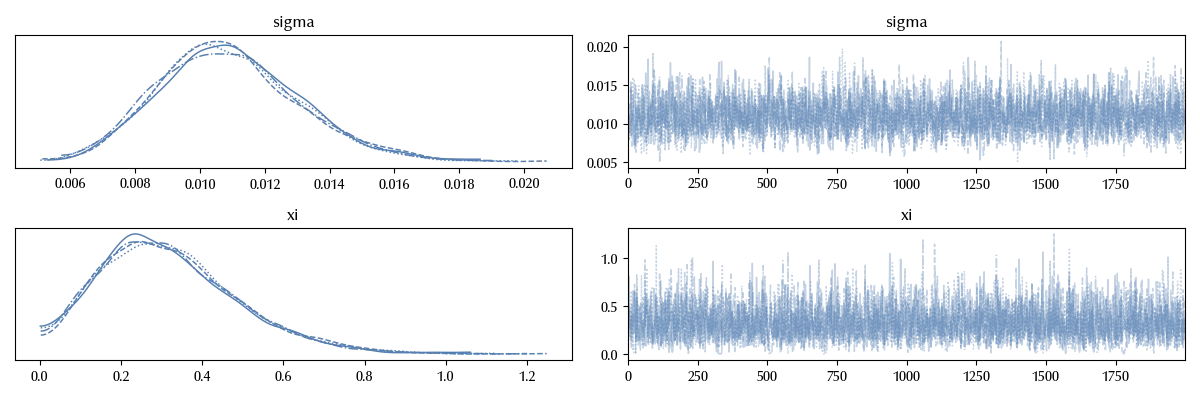
Notice that in our model we fixed $\mu$ to the threshold, which is fixed.

with pareto_model:
    ppc_pareto = pm.sample_posterior_predictive(trace_pareto, random_seed=rng)

fig = plt.figure()
ax = fig.add_subplot(111)
az.plot_ppc(ppc, ax=ax, mean=False, num_pp_samples=500)
ax.set_xlim([thr, 0.3])

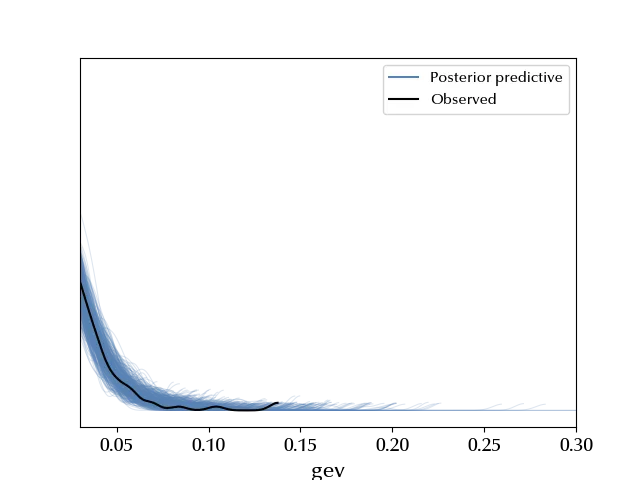
The posterior predictive of the Pareto model

In the last figure, the mean has been removed as Arviz has some issues in computing the mean for this posterior predictive, probably because of the heavy tails or due to the discontinuity at the threshold. Regardless from this, the agreement between the posterior predictive and the data looks perfect.

Conclusions

We introduced the Extreme Value theory, and we first applied it by fitting the weekly minima of the Apple stocks by using the GEV distribution. We then showed how to fit the data above a fixed threshold by using the generalized Pareto distribution.

Maximum distribution of the Apple stocks

The Generalized Pareto distribution

Conclusions

Suggested readings