Frailty models and cure rate models

In this post we will introduce frailty models and cure rate models, and we will show how to implement them in PyMC.

Frailty models

In many applications, the risk function may depend on unobserved or even unknown risk factors, and an individual’s risk factor is known as frailty or heterogeneity. Frailty models allow to model the association among unknown risk factors between different subpopulations, and there are many ways to account for frailties. Here we will show how to implement a frailty Weibull model with additive frailties.

import numpy as np
import pandas as pd
import pymc as pm
import arviz as az
from matplotlib import pyplot as plt
from SurvSet.data import SurvLoader


rng = np.random.default_rng(20251025)
loader = SurvLoader()

kwargs = dict(
    draws=2500,
    tune=2500,
    chains=4,
    nuts_sampler='nutpie',
    random_seed=rng
)

df, ref = loader.load_dataset(ds_name = 'Dialysis').values()

The dataset

As can be seen by ref, the dataset comes from an analysis of Sa Carvalho et al. (2003) of a sample of 6805 patients in Rio de Janeiro, and a more extensive description of the dataset can be found at this link. Here we will focus on a subset of patients affected by hypertension.

The sample is composed by patients coming from 67 different hospitals, and it is natural to assume that the hospital can have an effect on the survival probability of the patient. A frailty model looks a natural way to account for this effect, and we will therefore use this model to analyze the dataset.

Implementation

df_sel = df[df['fac_disease']=="hypert"].copy()

df_sel['censoring'] = [None if event else time for time, event in zip(df_sel['time'], df_sel['event'])]

df_sel['fac_center'] = pd.Categorical(df_sel['fac_center'])

with pm.Model(coords={'obs': df_sel.index, 'center': df_sel['fac_center'].drop_duplicates()}) as model:
    Xage = pm.Data('Xage', (df_sel['num_age']-df_sel['num_age'].mean())/(2*df_sel['num_age'].std()), dims=('obs'))
    mu = pm.Normal('mu', mu=0, sigma=2)
    sigma = pm.HalfNormal('sigma', sigma=2)
    eta = pm.Normal('eta', mu=0, sigma=1, dims=('center'))
    alpha = pm.Deterministic('alpha', mu+sigma*eta, dims=('center'))
    beta = pm.Normal('beta', mu=0, sigma=10)
    delta = pm.Normal('delta', mu=0, sigma=0.5)
    dist = pm.Weibull.dist(alpha=pm.math.exp(alpha[df_sel['fac_center'].cat.codes] + delta*Xage ), beta=pm.math.exp(beta))
    y = pm.Censored('y', dist=dist, lower=None, upper=df_sel['censoring'], observed=df_sel['time'], dims=('obs'))


with model:
    idata = pm.sample(**kwargs)
    
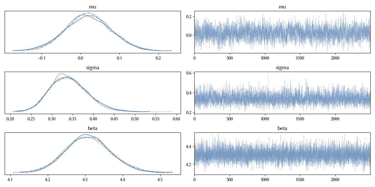
az.plot_trace(idata, var_names=['mu', 'sigma', 'beta'])
fig = plt.gcf()
fig.tight_layout()

The trace of our model

az.plot_forest(idata, var_names=['alpha'], combined=True)
fig = plt.gcf()
fig.tight_layout()

The hospital effect

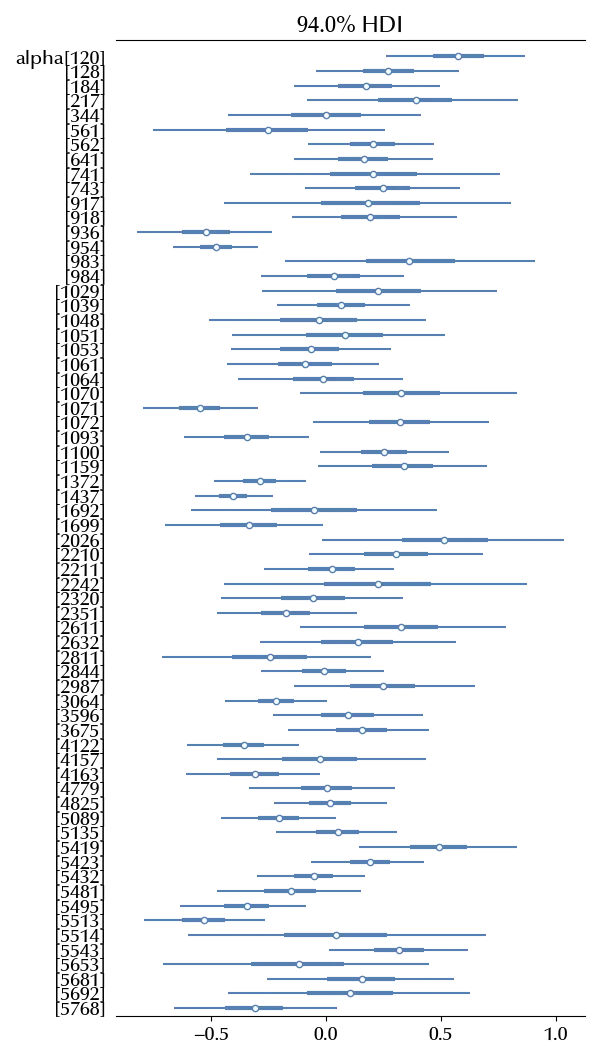
From the above plot it is clear that we should account for the hospital effect in order to properly quantify the expected patient’s survival time.

Cure rate model

Up to now we assumed that the event, soon or late, had to occur, but is many situations this assumption can be relaxed, and this is the main idea behind cure rate models. This model assumes that the survival function of the entire population is given by

\[S_{1}(t) = (1-\pi) + \pi S^*(t)\]

where $1-\pi$ is the fraction of cured population, and $S^*(t)$ is the survival function of the non-cured population. It can be shown (see these notes) that the general likelihood function for the mixture rate model can be written as

\[L = (\pi f^*_\theta(t))^{\delta_i} (\pi S^*_\theta(t) + (1-\pi))^{1-\delta_i}\]

The implementation is straightforward using pm.Potential(), as we will show in the following

Implementing the cure rate model

Let us switch to the E1684 dataset, that we already used in this example.

df_cr, ref_cr = loader.load_dataset(ds_name='e1684').values()

time, survival_prob, conf_int = kaplan_meier_estimator(
    df_cr["event"].astype(bool), df_cr['time'], conf_type="log-log"
)

fig, ax = plt.subplots()
ax.step(time, survival_prob, where="post", color='C0')
fig.tight_layout()

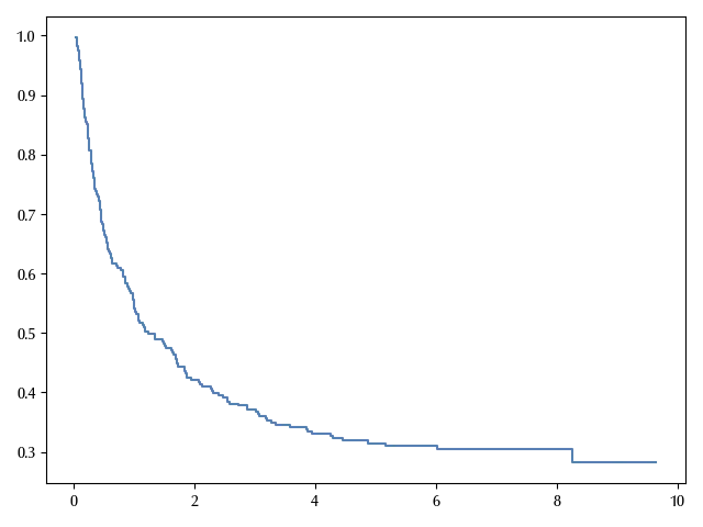
The Kaplan-Meier estimator for the entire population

From the above figure, it might be reasonable to assume that the survival function does not approach 0, but it rather saturates at some positive value, so a cure rate model seems appropriate for this dataset.

with pm.Model() as cure_rate_model:
    alpha = pm.Gamma('alpha', alpha=0.01, beta=0.01)
    beta = pm.Gamma('beta', alpha=0.01, beta=0.01)
    pi = pm.Uniform('pi')
    dist = pm.Weibull.dist(alpha=alpha, beta=beta)
    
    def logp(nu, y):
        return (nu*(pm.logp(dist, y) + pm.math.log(pi))
        + (1-nu)*pm.math.log((1-pm.math.exp(pm.logcdf(dist, y)))*pi + (1-pi)))
    y = pm.Potential('y', logp(df_cr['event'].values, df_cr['time'].values))

with cure_rate_model:
    idata_cr = pm.sample(**kwargs)

az.plot_trace(idata_cr, var_names=['alpha', 'beta', 'pi'])
fig = plt.gcf()
fig.tight_layout()

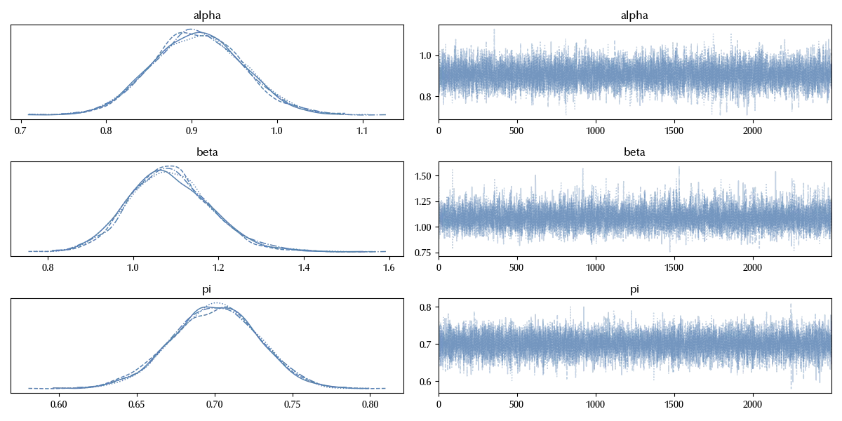
In the above model, $1-\pi$ represents the fraction of cured population, so it represents the asymptotic value of $S_1(t)$, and this looks compatible with the value of 0.7 that the cure rate model is giving us.

Conclusions

Frailty models can be used to account for the association of unknown risk factors among groups, and they are appropriate when you expect that the risk function depends on unobserved factors which vary between subgroups in your sample.

On the other hand, cure rate models can be used to take into account for units which will never experience the event, and they can be easily implemented in PyMC.