

Accelerated Failure Time models
All models are wrong, but there are situations when one may be less wrong than another. Here we will discuss Accelerated Failure Time survival models, which are another popular family of models in survival analysis. AFT models assume that the effect of the covariates is to increase the speed the course of the disease by some factor.
As we did in our previous post, we will only consider the treatment effect and neglect any other factor, but the generalization to any factor is straightforward.
We will again use the melanoma dataset, and in our discussion we will stick to the Weibull model.
The AFT Weibull model in PyMC has been extensively discussed in this post, and in the references therein, while a more in-depth mathematical discussion can be found in this article.
The Gumbel distribution
Let us take a random Weibull distribution $t$,
\[t \sim W(\alpha, \beta)\,,\]As shown in the above reference, its logarithm is then distributed according to a Gumbel (also known as log-Weibull) distribution
\[\log(t) \sim G(\log(\beta), 1/\alpha)\,.\]Since in AFT model we assume that the effect of the covariates is multiplicative on the time, then it must be additive on the log-time. In order to implement a Weibull AFT model, we must only include the covariates effect into the location parameter of the Gumbel distribution.
Let us try and implement it, and let us compare it with our previous Weibull survival model.
import numpy as np
import pandas as pd
import pymc as pm
import arviz as az
from matplotlib import pyplot as plt
from SurvSet.data import SurvLoader
from scipy.special import gammaln
import pytensor as pt
from sksurv.nonparametric import kaplan_meier_estimator

rng = np.random.default_rng(6543)
loader = SurvLoader()

df_melanoma, ref_melanoma = loader.load_dataset(ds_name = 'e1684').values()

df_melanoma['log_time'] = np.log(df_melanoma['time'])

df_melanoma['trt'] = (df_melanoma['fac_trt']=='IFN').astype(int)

df_melanoma['censoring'] = [None if x==1 else y for x, y in zip(df_melanoma['event'], df_melanoma['time'])]
df_melanoma['acc_censoring'] = [None if x==1 else y for x, y in zip(df_melanoma['event'], df_melanoma['log_time'])]

with pm.Model() as weibull_model:
    alpha = pm.Normal('alpha', mu=0, sigma=100)
    beta = pm.Normal('beta', mu=0, sigma=100, shape=2)
    lam = pm.math.exp(beta[0] + beta[1]*df_melanoma['trt'])
    dist = pm.Weibull.dist(alpha=pm.math.exp(alpha), beta=lam)
    y = pm.Censored('y', dist, lower=None, upper=df_melanoma['censoring'], observed=df_melanoma['time'])

with weibull_model:
    idata_weibull = pm.sample(nuts_sampler='numpyro', draws=2000, random_seed=rng)

az.plot_trace(idata_weibull)
fig = plt.gcf()
fig.tight_layout()
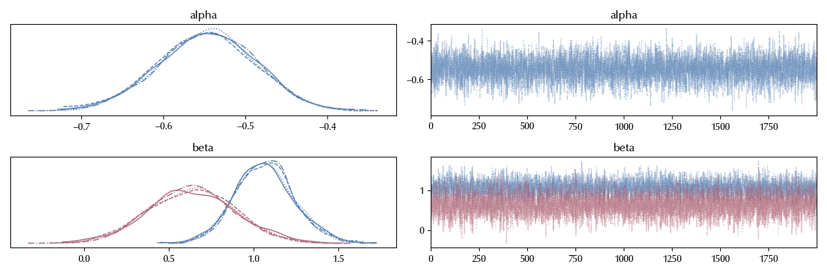
Up to now, we only re-performed tha same calculations we did in our old post. Let us now implement the AFT Weibull model.
with pm.Model() as aft_weibull_model:
    alpha = pm.Normal('alpha', mu=0, sigma=100)
    beta = pm.Normal('beta', mu=0, sigma=100, shape=2)
    lam = pm.math.exp(alpha)
    mu = beta[0] + beta[1]*df_melanoma['trt']
    dist = pm.Gumbel.dist(mu=mu, beta=lam)
    y = pm.Censored('y', dist, lower=None, upper=df_melanoma['acc_censoring'], observed=df_melanoma['log_time'])

with aft_weibull_model:
    idata_weibull_aft = pm.sample(nuts_sampler='numpyro', draws=2000, random_seed=rng)

az.plot_trace(idata_weibull_aft)
fig = plt.gcf()
fig.tight_layout()
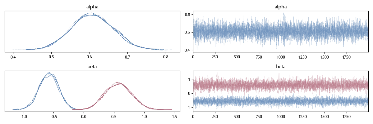
Also in this case, the trace looks ok. We must now only compare the models and decide which one is better. Using the LOO would however be a bad idea, since in one model we are fitting the survival time, while in the other model we are fitting its logarithm, and this would make impossible a comparison of the log-likelihoods of the two models.
We will therefore use a visual inspection to perform the comparison.
def Sw(t, alpha, beta):
    y = (t/beta)**alpha
    return np.exp(-y)

def Sg(y, mu, sig):
    return 1. - np.exp(-np.exp(-(y - mu) / sig))

df0 = df_melanoma[df_melanoma['trt']==0]
df1 = df_melanoma[df_melanoma['trt']==1]

time0, survival_prob0, conf_int0 = kaplan_meier_estimator(
    df0["event"].astype(bool), df0['time'], conf_type="log-log"
)

time1, survival_prob1, conf_int1 = kaplan_meier_estimator(
    df1["event"].astype(bool), df1['time'], conf_type="log-log"
)

t_pl =  np.arange(0.02, 10, 0.02)

alph = np.exp(idata_weibull.posterior['alpha'].values.reshape(-1))
b0 = np.exp(idata_weibull.posterior['beta'].values.reshape(-1,2)[:, 0])
b1 = np.exp(idata_weibull.posterior['beta'].values.reshape(-1,2)[:, 0]+idata_weibull.posterior['beta'].values.reshape(-1,2)[:, 1])

s0 = [np.mean(Sw(t, alph, b0)) for t in t_pl]
s0_low = [np.quantile(Sw(t, alph, b0), q=0.03) for t in t_pl]
s0_high = [np.quantile(Sw(t, alph, b0), q=0.97) for t in t_pl]

s1 = [np.mean(Sw(t, alph, b1)) for t in t_pl]
s1_low = [np.quantile(Sw(t, alph, b1), q=0.03) for t in t_pl]
s1_high = [np.quantile(Sw(t, alph, b1), q=0.97) for t in t_pl]

alpha = np.exp(idata_weibull_aft.posterior['alpha'].values.reshape(-1))
b0a = idata_weibull_aft.posterior['beta'].values.reshape(-1,2)[:, 0]
b1a = idata_weibull_aft.posterior['beta'].values.reshape(-1,2)[:, 0]+idata_weibull_aft.posterior['beta'].values.reshape(-1,2)[:, 1]

s0a = [np.mean(Sg(np.log(t), b0a, alpha)) for t in t_pl]
s0a_low = [np.quantile(Sg(np.log(t),b0a, alpha), q=0.03) for t in t_pl]
s0a_high = [np.quantile(Sg(np.log(t), b0a, alpha), q=0.97) for t in t_pl]

s1a = [np.mean(Sg(np.log(t), b1a, alpha)) for t in t_pl]
s1a_low = [np.quantile(Sg(np.log(t),b1a, alpha), q=0.03) for t in t_pl]
s1a_high = [np.quantile(Sg(np.log(t), b1a, alpha), q=0.97) for t in t_pl]

fig, ax = plt.subplots(ncols=2, sharey=True, figsize=(12, 4))
ax[0].plot(t_pl, s0, label='Weibull', color='C0')
ax[0].plot(t_pl, s0a, label='AFT', color='C1')
ax[0].step(time0, survival_prob0, where="post", color='gray')

ax[1].plot(t_pl, s1, label='Weibull', color='C0')
ax[1].plot(t_pl, s1a, label='AFT', color='C1')
ax[1].step(time1, survival_prob1, where="post", color='gray')

ax[0].set_ylim([0, 1])
ax[0].set_xlim([0, t_pl[-1]])
ax[1].set_xlim([0, t_pl[-1]])

ax[0].set_title(f'$S_0(t)$')
ax[1].set_title(f'$S_1(t)$')
ax[0].legend(frameon=False)
ax[1].legend(frameon=False)
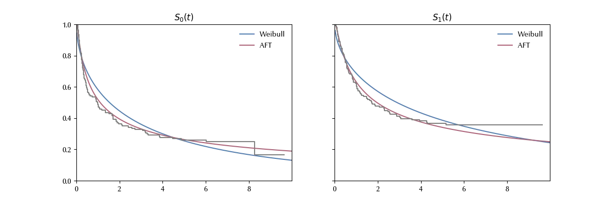
The AFT model shows a better agreement with the data with respect to the old model. This often happens when the study subject is a biological survival process, but one should always compare the models and choose the most appropriate for the question under study.
Conclusions
Accelerated Failure Time models are a popular tool in survival analysis, and here we discussed how to implement them in PyMC.
%load_ext watermark
%watermark -n -u -v -iv -w -p xarray,numpyro,jax,jaxlib
Python implementation: CPython
Python version : 3.12.8
IPython version : 8.31.0
xarray : 2025.1.1
numpyro: 0.16.1
jax : 0.5.0
jaxlib : 0.5.0
SurvSet : 0.2.6
matplotlib: 3.10.1
arviz : 0.21.0
pytensor : 2.30.3
numpy : 2.1.3
pandas : 2.2.3
sksurv : 0.24.1
pymc : 5.22.0
Watermark: 2.5.0