Application of survival analysis 1

In the previous post we introduced survival analysis, and we discussed how to correctly treat censorship. In this post we will see an application of survival analysis.

The study

In this post we will use the “E1684” melanoma dataset available in the SurvSet python package.

import numpy as np
import pandas as pd
import pymc as pm
import arviz as az
from matplotlib import pyplot as plt
from SurvSet.data import SurvLoader
from scipy.special import gammaln
import pytensor as pt
from sksurv.nonparametric import kaplan_meier_estimator


rng = sum(map(ord,'survival_example'))

kwargs=dict(nuts_sampler='nutpie',
                           draws=5000, random_seed=rng)

loader = SurvLoader()

df_melanoma, ref_melanoma = loader.load_dataset(ds_name = 'e1684').values()

# Dataset reference

ref_melanoma

https://www.rdocumentation.org/packages/smcure/versions/2.0/topics/e1684

df_melanoma.head()

	pid	event	time	num_age	fac_sex	fac_trt
0	0	1	1.15068	-11.0359	0	1
1	1	1	0.62466	-5.12904	0	1
2	2	0	1.89863	23.186	1	0
3	3	1	0.45479	11.1449	1	0
4	4	1	2.09041	-13.3208	0	0

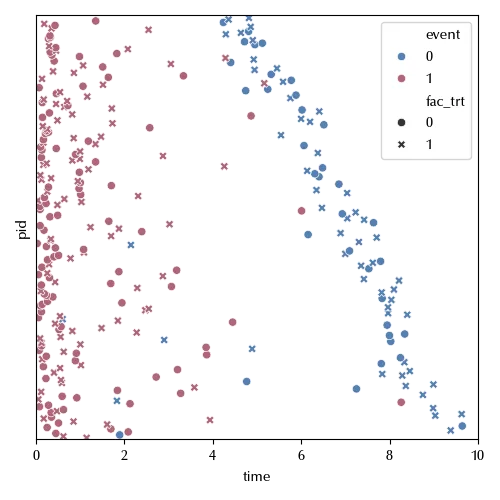
There variable “time” is our regression variable, the “event” column indicates if the event happened, and its value is 1 if the event happened (the patient died) while it is 0 if the event is censored.

len(df_melanoma)

284

Let us count how many entries are censored

(df_melanoma['event']==0).astype(int).sum()

df_melanoma['time'].max()

9.64384

We can now try and visually inspect the dataset.

fig, ax = plt.subplots(figsize=(5, 5))
sns.scatterplot(df_melanoma, y='pid', x='time', hue='event', style='fac_trt')
ax.set_yticks([])
ax.set_ylim([-1, 1+len(df_melanoma)])
ax.set_xlim([0, 10])
fig.tight_layout()

The scatterplot of the dataset

The models

We will try and fit two models: first we will try with an Exponential likelihood,

\[Y \sim \mathcal{Exponential}(\lambda)\]

we will then try with a Weibull likelihood, which is a quite flexible distribution, which allows for fatter tails, and it should thereby be more robust than an exponential or a Gamma distribution.

\[Y \sim \mathcal{Weibull}(\sigma, \lambda)\]

The Weibull distribution has pdf

\[p(x | \alpha, \lambda) = \alpha \frac{x^{\alpha-1}}{\lambda^\alpha} e^{-(x/\lambda)^\alpha}\]

Notice that, often, the second parameter is named $\beta$, but since we will use this method for another purpose, we will use $\lambda$ for the second parameter. Both the parameters must be positive, and the mean of the distribution is

\[\mu = \lambda \Gamma\left(1+\alpha^{-1}\right)\]

We want to assess the effectiveness of the treatment. The first possibility is to fit two different models, one per treatment. Another very common possibility is to use the treatment as a regression variable, and we will use this method. We assume

\[\begin{align} & \lambda = \exp\left(\beta_0 + \beta_1 x \right) \\ & \sigma = \exp\left(\alpha \right) \\ & \alpha, \beta_i \sim \mathcal{N}(0, 100) \\ \end{align}\]

In this way we ensure that both the parameters are positive, and the priors are very uninformative. Let us introduce the censoring variable

df_melanoma['censoring'] = [None if x==1 else y for x, y in zip(df_melanoma['event'], df_melanoma['time'])]

We will first try with the exponential model, as discussed in chapter 2 of “Bayesian Survival Analysis”

with pm.Model() as expon_model:
    beta = pm.Normal('beta', mu=0, sigma=1000, shape=2)
    lam = pm.math.exp(beta[0] + beta[1]*df_melanoma['fac_trt'])
    dist = pm.Exponential.dist(lam=lam)
    y = pm.Censored('y', dist, lower=None, upper=df_melanoma['censoring'],
                    observed=df_melanoma['time'])
    idata_expon = pm.sample(**kwargs)

az.plot_trace(idata_expon)
fig = plt.gcf()
fig.tight_layout()

The trace of the exponential model model

The image is similar, but not identical to the one of the reference. However, our model is identical to the one provided in the reference. In order to check this, you can try and fit the following model:

with pm.Model() as expon_model_check:
    beta = pm.Normal('beta', mu=0, sigma=1000, shape=2)
    lam = pm.math.exp(beta[0] + beta[1]*df_melanoma['fac_trt'])
    def logp(lam, nu, y):
        return nu*pm.math.log(lam)-y*lam
    y = pm.Potential('y', logp(lam, df_melanoma['event'].values, df_melanoma['time'].values))

with expon_model_check:
    idata_check = pm.sample(**kwargs)

The formula for the log-likelihood is the one provided in the reference. If you try and fit the model, you will get exactly the same figure we obtained. The reason for the different trace is, probably, that the samplers improved quite a lot in more than 20 years, in fact our trace looks much better than the one in the reference.

We will now improve our model and try with the Weibull model

with pm.Model() as weibull_model:
    alpha = pm.Normal('alpha', mu=0, sigma=100)
    beta = pm.Normal('beta', mu=0, sigma=100, shape=2)
    lam = pm.math.exp(beta[0] + beta[1]*df_melanoma['fac_trt'])
    dist = pm.Weibull.dist(alpha=pm.math.exp(alpha), beta=lam)
    y = pm.Censored('y', dist, lower=None, upper=df_melanoma['censoring'],
                    observed=df_melanoma['time'])

with weibull_model:
    idata_weibull = pm.sample(**kwargs)

az.plot_trace(idata_weibull)
fig = plt.gcf()
fig.tight_layout()

The trace of the Weibull model model

As we discussed, when you have two nested model, it is generally better to use the more general one. We will however try and compare the models in order to see which is the more appropriate

with expon_model:
    pm.compute_log_likelihood(idata_expon)

with weibull_model:
    pm.compute_log_likelihood(idata_weibull)

with expon_model:
    idata_expon.extend(pm.sample_posterior_predictive(idata_expon, random_seed=rng))

with weibull_model:
    idata_weibull.extend(pm.sample_posterior_predictive(idata_weibull, random_seed=rng))

df_compare = az.compare({'Exponential': idata_expon, 'Weibull': idata_weibull})

az.plot_compare(df_compare)
fig = plt.gcf()
fig.tight_layout()

The LOO model comparison

The Weibull model seems much more appropriate to describe the data, we will therefore stick to it from now on.

Treatment comparison

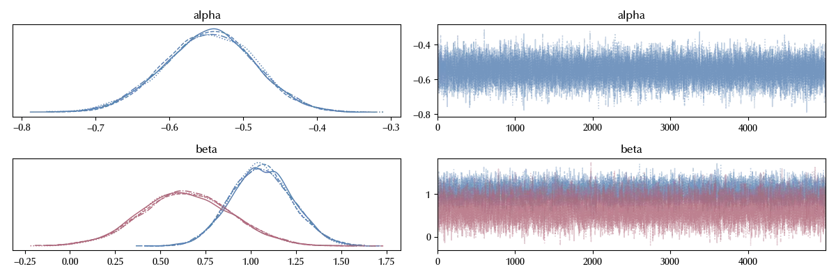
By looking at the Weibull trace, we observe that $\beta_1>0\,,$ and this indicates that the test treatment is more effective than the control one. This becomes clearer by showing the distribution of the mean $\mu$

with weibull_model:
    mu0 = pm.Deterministic('mu0', pm.math.exp(beta[0])*pm.math.exp(pt.tensor.math.gammaln(1+1/pm.math.exp(alpha))))
    mu1 = pm.Deterministic('mu1', pm.math.exp(beta[0]+beta[1])*pm.math.exp(pt.tensor.math.gammaln(1+1/pm.math.exp(alpha))))

with weibull_model:
    idata_mu = pm.sample_posterior_predictive(idata_weibull, var_names=['mu0', 'mu1'])

fig, ax = plt.subplots(nrows=2)
xlim = [2, 15]
az.plot_posterior(idata_mu, group='posterior_predictive', var_names='mu0', ax=ax[0])
az.plot_posterior(idata_mu, group='posterior_predictive', var_names='mu1', ax=ax[1])
ax[0].set_xlim(xlim)
ax[1].set_xlim(xlim)
ax[0].set_title("$\\mu_0$")
ax[1].set_title("$\\mu_1$")
fig.tight_layout()

The posterior for the parameter mu

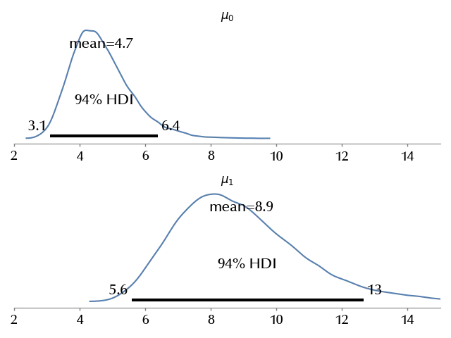
The mean for the test treatment is typically higher for the test group than for the control group, and the peak of the mean for the IFN treatment is roughly twice than the one for the control treatment.

Let us also take a look at the survival function, which is simply

\[S(t, \alpha, \beta) = e^{-(t/\beta)^\alpha}\]

We will also compare the survival function obtained from our model with the Kaplan-Meier estimator of the survival function

df0 = df_melanoma[df_melanoma['fac_trt']==0]
df1 = df_melanoma[df_melanoma['fac_trt']==1]

time0, survival_prob0, conf_int0 = kaplan_meier_estimator(
    df0["event"].astype(bool), df0['time'], conf_type="log-log"
)

time1, survival_prob1, conf_int1 = kaplan_meier_estimator(
    df1["event"].astype(bool), df1['time'], conf_type="log-log"
)
def S(t, alpha, beta):
    y = (t/beta)**alpha
    return np.exp(-y)

t_pl =  np.arange(0., 10, 0.02)

alph = np.exp(idata_weibull.posterior['alpha'].values.reshape(-1))
b0 = np.exp(idata_weibull.posterior['beta'].values.reshape(-1,2)[:, 0])
b1 = np.exp(idata_weibull.posterior['beta'].values.reshape(-1,2)[:, 0]+idata_weibull.posterior['beta'].values.reshape(-1,2)[:, 1])

s0 = [np.mean(S(t, alph, b0)) for t in t_pl]
s0_low = [np.quantile(S(t, alph, b0), q=0.03) for t in t_pl]
s0_high = [np.quantile(S(t, alph, b0), q=0.97) for t in t_pl]

s1 = [np.mean(S(t, alph, b1)) for t in t_pl]
s1_low = [np.quantile(S(t, alph, b1), q=0.03) for t in t_pl]
s1_high = [np.quantile(S(t, alph, b1), q=0.97) for t in t_pl]

fig, ax = plt.subplots(ncols=2, sharey=True, figsize=(12, 4))
ax[0].plot(t_pl, s0, label='Control', color='C0')
ax[0].fill_between(t_pl, s0_low, s0_high, alpha=0.5, color='lightgray')
ax[0].step(time0, survival_prob0, where="post", color='C0')
ax[1].step(time1, survival_prob1, where="post", color='C1')
ax[1].plot(t_pl, s1, label='IFN', color='C1')
ax[0].fill_between(time0, conf_int0[0], conf_int0[1], alpha=0.25, step="post", color='C0')
ax[1].fill_between(time1, conf_int1[0], conf_int1[1], alpha=0.25, step="post", color='C1')
ax[1].fill_between(t_pl, s1_low, s1_high, alpha=0.5, color='lightgray')
ax[0].set_ylim([0, 1])
ax[0].set_xlim([0, t_pl[-1]])
ax[1].set_xlim([0, t_pl[-1]])

ax[0].set_title(f'$S_0(t)$')
ax[1].set_title(f'$S_1(t)$')
ax[0].legend(frameon=False)
ax[1].legend(frameon=False)

The survival functions

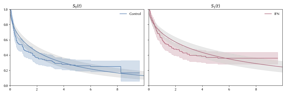
We can safely conclude that, for the patients in this study, the IFN treatment gives better results than the control one.

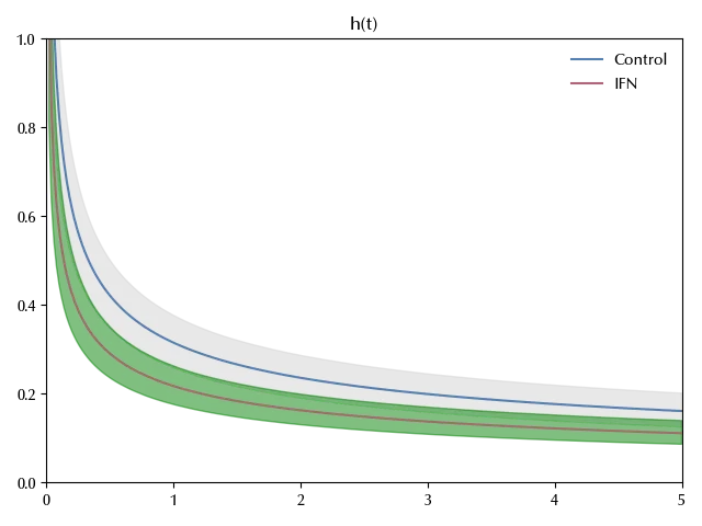
Also the hazard function can be easily computed:

def h(t, alpha, beta):
    y = alpha*(t/beta)**(alpha)/t
    return y

t_pl =  np.arange(0.02, 5, 0.02)


h0 = [np.mean(h(t, alph, b0)) for t in t_pl]
h0_low = [np.quantile(h(t, alph, b0), q=0.03) for t in t_pl]
h0_high = [np.quantile(h(t, alph, b0), q=0.97) for t in t_pl]

h1 = [np.mean(h(t, alph, b1)) for t in t_pl]
h1_low = [np.quantile(h(t, alph, b1), q=0.03) for t in t_pl]
h1_high = [np.quantile(h(t, alph, b1), q=0.97) for t in t_pl]

fig = plt.figure()
ax = fig.add_subplot(111)
ax.plot(t_pl, h0, label='Control')
ax.fill_between(t_pl, h0_low, h0_high, alpha=0.5, color='lightgray')

ax.plot(t_pl, h1, label='IFN')
ax.fill_between(t_pl, h1_low, h1_high, alpha=0.5, color='green')
ax.set_ylim([0, 1])
ax.set_xlim([0, t_pl[-1]])

ax.set_title(f'h(t)')
legend = plt.legend(frameon=False)

The hazard functions obtained from our model

Conclusions

We discussed an application of survival analysis with continuous time, we explained how to include the regressor dependence in bayesian survival analysis, and we also introduced the Weibull distribution.

In the next post, we will discuss a more flexible way to estimate the survival function.

The study

The models

Treatment comparison

Conclusions

Suggested readings