Application of survival analysis with discrete times

In the last example, we discussed how to perform a survival analysis by providing a family for the survival function $S\,.$ This method provides strong constraints to the form of the survival function and to the related quantities, but sometimes you might need more flexibility. In this post we will see an alternative model, which gives you more flexibility. While the previous method, however, treated the time as a continuous quantity, the method discussed in this section makes the time discrete.

Survival analysis with logistic regression

In this example, we will discuss an application I encountered some time ago. This kind of method can be found in many textbooks, but I will stick to this article by Efron, which has been discussed in this blog post.

In this model we assume that the number of survived individuals follows a binomial distribution

\[y_i \vert n_i, h_i \sim \mathcal{Binom}(h_i, n_i)\]

Here $h_i$ represents the hazard function evaluated at time $t_i\,.$ Within this framework, the survival function is related to the hazard function via

\[S_i = \prod_{j\leq i} (1-h_i)\,.\]

In the logistic regression, one assumes

\[h_i = \frac{1}{1+e^{\phi(t_i)}}\,.\]

In the paper, Efrom assumes that

\[\phi(t_i) = \beta_0 + \beta_1 t_i + \beta_2 (t_i-11)_{-}^2+ \beta_3 (t_i-11)_{-}^3\]

where

\[(x)_{-} = \begin{cases} x & \, if\, \, x<0\\ 0 & \, if\, \, x\geq0\\ \end{cases}\]

As explained in the article, the above choice allows for structure at the beginning of the study, when data is collected often and carefully, while the later stages are assumed to be linear.

Implementing the model

We took the datasets from the blog.

import pandas as pd
import pymc as pm
import arviz as az
import numpy as np
from matplotlib import pyplot as plt

rng = np.random.default_rng(sum(map(ord,'example_2')))

df = pd.read_csv('./survival_efron.csv')

df_1 = pd.read_csv('./survival_efron_1.csv')

kwargs=dict(nuts_sampler='numpyro', random_seed=rng, tune=5000, draws=5000, target_accept=0.9)

Let us now implement the necessary functions

def f1(x):
    y = x-11
    return np.minimum(y, y*0)**2

def f2(x):
    y = x-11
    return np.minimum(y, y*0)**3

We can now build the regression variables

X_f = df[['month']].rename(columns={'month': 't'})
X_f['t2'] = f1(X_f['t'])
X_f['t3'] = f2(X_f['t'])

X1_f = df_1[['month']].rename(columns={'month': 't'})
X1_f['t2'] = f1(X1_f['t'])
X1_f['t3'] = f2(X1_f['t'])

We are now ready to implement the model for the first dataset

coords = {'obs': X_f.index, 'cols': X_f.columns}

with pm.Model(coords=coords) as efron:
    n = pm.Data('n', df['n'], dims=['obs'])
    X = pm.Data('X', X_f, dims=['obs', 'cols'])
    beta = pm.Normal('beta', mu=0, sigma=1, dims=['cols'])
    alpha = pm.Normal('alpha', mu=0, sigma=3)
    lam = pm.Deterministic('lam', alpha+pm.math.dot(beta, X.T))
    h = pm.Deterministic('h', pm.math.invlogit(lam))
    g = pm.Deterministic('g', pm.math.cumprod(1-h))
    y = pm.Binomial('y', p=h, n=n, observed=df['s'], dims=['obs'])

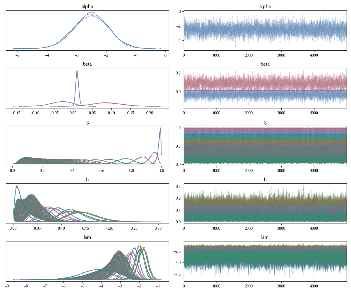
with efron:
    idata = pm.sample(**kwargs)

az.plot_trace(idata)
fig = plt.gcf()
fig.tight_layout()

The trace of the first model

Similarly

coords1 = {'obs': X1_f.index, 'cols': X1_f.columns}

with pm.Model(coords=coords1) as efron1:
    n = pm.Data('n', df_1['n'], dims=['obs'])
    X = pm.Data('X', X1_f, dims=['obs', 'cols'])
    beta = pm.Normal('beta', mu=0, sigma=1, dims=['cols'])
    alpha = pm.Normal('alpha', mu=0, sigma=3)
    lam = pm.Deterministic('lam', alpha+pm.math.dot(beta, X.T))
    h = pm.Deterministic('h', pm.math.invlogit(lam))
    g = pm.Deterministic('g', pm.math.cumprod(1-h))
    y = pm.Binomial('y', p=h, n=n, observed=df_1['s'], dims=['obs'])

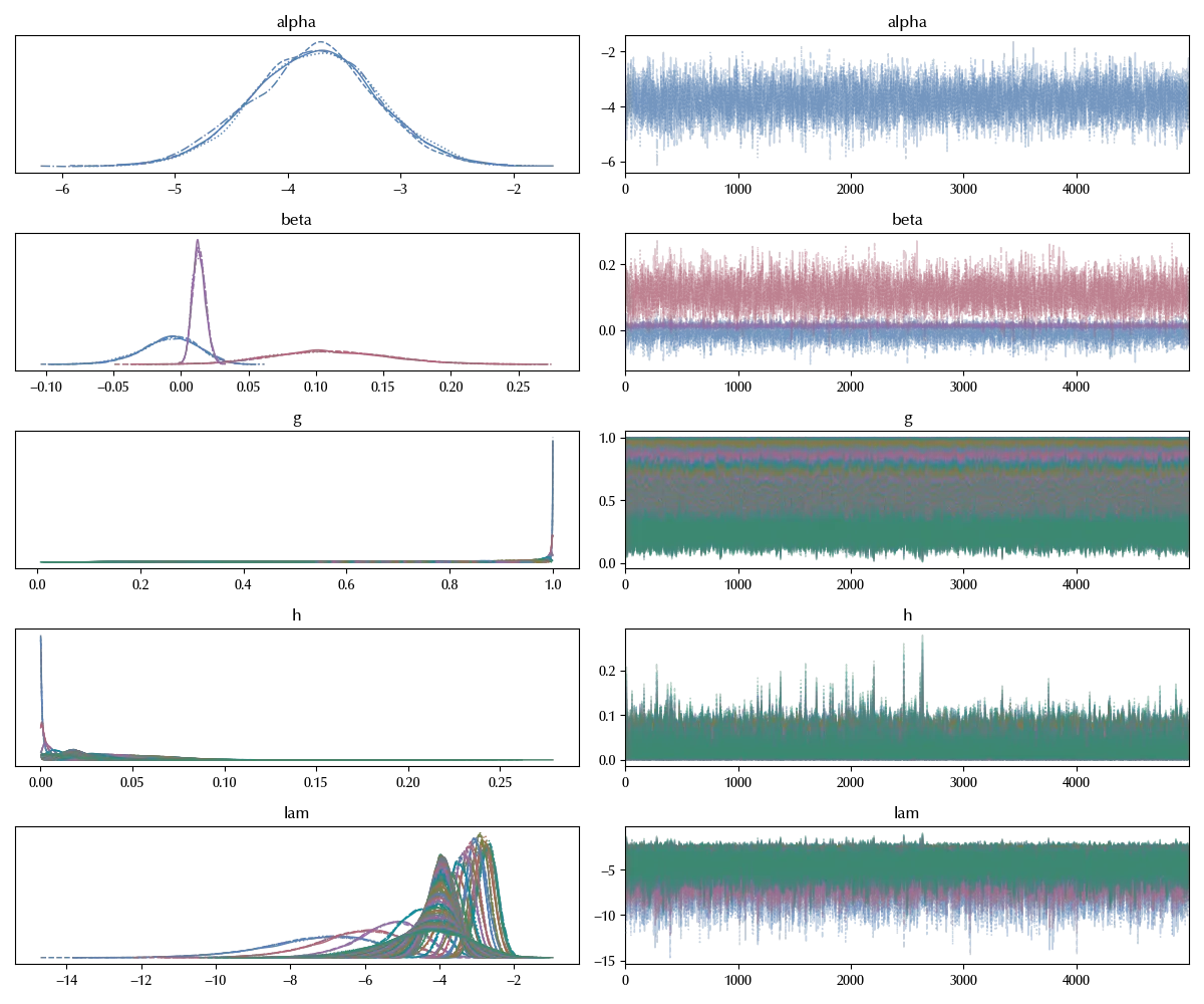
with efron1:
    idata1 = pm.sample(**kwargs)

az.plot_trace(idata1)
fig = plt.gcf()
fig.tight_layout()

The trace of the second model

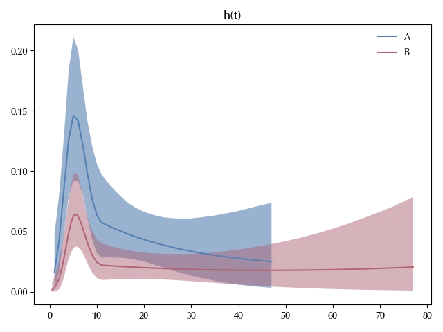
We can now plot our estimates for the hazard functions

fig = plt.figure()
ax = fig.add_subplot(111)
ax.fill_between(X_f['t'], idata.posterior['h'].quantile(q=0.03, dim=('draw', 'chain')),
                idata.posterior['h'].quantile(q=0.97, dim=('draw', 'chain')), alpha=0.6)
ax.plot(X_f['t'], idata.posterior['h'].mean(dim=('draw', 'chain')), label='A')
ax.fill_between(X1_f['t'], idata1.posterior['h'].quantile(q=0.03, dim=('draw', 'chain')),
                idata1.posterior['h'].quantile(q=0.97, dim=('draw', 'chain')), alpha=0.5)
ax.plot(X1_f['t'], idata1.posterior['h'].mean(dim=('draw', 'chain')), label='B')
ax.set_title(f"h(t)")
legend = fig.legend(loc='upper right',  borderaxespad=3, frameon=False)
fig.tight_layout()

Our estimate for the hazard functions

We can also plot the survival functions. It is instructive to compare our estimates with the so-called Kaplan Meier estimator, which is a non-parametric estimator of the survival function:

\[S_{KM}(t_i) = \prod_{j \leq i} \left(1-\frac{y_j}{n_j}\right)\,.\]

ym = idata.posterior['g'].mean(dim=('draw', 'chain'))
yl = idata.posterior['g'].quantile(q=0.03, dim=('draw', 'chain'))
yh = idata.posterior['g'].quantile(q=0.97, dim=('draw', 'chain'))

y1m = idata1.posterior['g'].mean(dim=('draw', 'chain'))
y1l = idata1.posterior['g'].quantile(q=0.03, dim=('draw', 'chain'))
y1h = idata1.posterior['g'].quantile(q=0.97, dim=('draw', 'chain'))

fig = plt.figure()
ax = fig.add_subplot(111)
ax.errorbar(X_f['t'], ym, yerr=[ym-yl, yh-ym], label='A')
ax.scatter(X_f['t'], np.cumprod(1- df['s']/df['n']), label='A KM')  # Kaplan Meier est.
ax.errorbar(X1_f['t'], y1m, yerr=[y1m-y1l, y1h-y1m], label='B')
ax.scatter(X1_f['t'], np.cumprod(1- df_1['s']/df_1['n']), label='B KM')  # Kaplan Meier est.
ax.set_xlim([0, 80])
ax.set_ylim([0, 1])
ax.set_title(f"S(t)")
legend = fig.legend(loc='upper right',  borderaxespad=5, frameon=False)

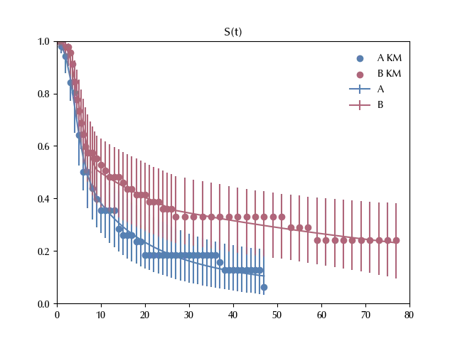
Our estimate for the survival functions

There is very good agreement with the two estimates, while it would be quite difficult to implement this flexibility with the tools we used in the last post.

Conclusions

The logistic regression can be a powerful tool to perform survival analysis, as it enable us to easily encode structure in a controlled and easily interpretable way.

Survival analysis with logistic regression

Implementing the model

Conclusions

Suggested readings