

Introduction to survival analysis
There are situations where your task is to estimate the waiting time before a certain event happens, and survival analysis is the branch of statistics which deals with this kind of study.
In general, time can be either considered a continuous variable or a discrete one. For the moment we will assume that it’s a continuous one.
Since we are dealing with a waiting time, our variable must be non-negative.
We will focus for now on parametric models, although non-parametric models are very popular in survival analysis.
The analyzed event can be either the time before a component fails or the occurrence of some biological change like the infection of one patient or even the next eruption of a volcano. This kind of model can be applied to a huge number of situations, from marketing to recruiting and even to house market, and it is useful when you want to estimate how long will it take to a client (or a resource) before leaving your company or how long will it take to you to sell a house.
Mathematical background
Let us consider a random variable $T$ with pdf $p$ and cumulative $F\,,$ we define the survival function $S$ as:
\[F(t) = P(t\leq T) = \int_0^t p(u) du = 1-S(t)\]We assume that at $t=0$ the event is not happened, so $S(0)=1$ while we assume that we are certain that the event must occur, so $\lim_{t\rightarrow \infty} S(t)=0\,.$
We may alternatively assume that the event does not happen with probability $p_0\,,$ and in this case we may modify the above assumption with $\lim_{t\rightarrow \infty} S(t)=p_0\,.$
We define the hazard function as
\[h(t) = \lim_{\Delta t \rightarrow 0} \frac{P(t< T \leq t+\Delta t | T>t)}{\Delta t} = \lim_{\Delta t \rightarrow 0} \frac{P((t< T \leq t+\Delta t) \cap T>t)}{P(T>t)\Delta t} = \lim_{\Delta t \rightarrow 0} \frac{P(t < T \leq t+\Delta t) }{\Delta t} \frac{1}{P(T>t)} = \frac{1}{S(t)}\lim_{\Delta t \rightarrow 0} \frac{F(t+\Delta t) - F(t)}{\Delta t }= \frac{F'(t)}{S(t)} = \frac{f(t)}{S(t)}\]Since $h$ is the ratio of two positive quantities, it is positive itself.
We have that
\[h(t) = \frac{f(t)}{S(t)} = -\frac{S'(t)}{S(t)} = -\frac{d}{dt}\log S(t)\]which can be inverted by first integrating and then exponentiating:
\[S(t) = \exp\left(-\int_0^t h(u) du\right)\]Notice that, if we assume that $\lim_{t\rightarrow \infty} S(t)=0\,,$ we must require that $\lim_{t\rightarrow \infty}\int_0^t h(u) du = \infty\,.$ If we otherwise assume that $\lim_{t\rightarrow \infty} S(t)=p_0\,,$ we must require that $\lim_{t\rightarrow \infty}\int_0^t h(u) du = -\log\left(p_0\right)\,.$
We define the cumulative hazard function as
\[H(t) = \int_0^t h(u) du\]And it is related to the survival function by
\[S(t) = \exp\left(-H(t)\right)\]Censoring
One of the main issues of survival analysis is that we are only able to observe our system for a finite amount of time $c$, and in this period the event may or may not occur.
Let us assume that we performed a study with duration $c\,,$ if we do not observe the event within the end of the study we cannot conclude that the event did not happen, we can only conclude that it did not happen within time $c$. We assume that the event must happen at some time. We introduce the outcome variable $y$ as \(y = \min(t, c)\) and define the censoring status variable $\delta$ which indicates if the event was observed or not
\[\delta = \begin{cases} 1\,\,\, if \,\,\, t < c \\ 0 \,\,\, if \,\,\, t \geq c \end{cases}\]and if it is not observed we say that it is censored. If the event is not censored then its contribution to the likelihood is, as usual, $f(t)\,,$ but if we do not observe the event within time $c$ then all we can conclude is that the event happened after time $c\,,$ and the probability for this is $S(c)\,.$ Thus the likelihood can be written as
\[L = f(y)^\delta S(y)^{1-\delta} = (h(y) S(y))^\delta S(y)^{1-\delta}= h(y)^\delta S(y)\]and this quantity is sometimes defined as the generalized likelihood.
As a practical example of censoring, I once received a dataset where the client gave me the start date and end date for a set of “practices” opened by his clients, together with a set of regressors, included the employee whom the practice was assigned, and I had to find insights on the average working time of the practice. The dataset also included rows where the end date was missing, and those were practices still in progress. We know that, sooner or later the practice will be closed, we simply did not wait enough to observe it, so we should consider those practices as censored.
Wrong methods for accounting of censoring
If you are new to survival analysis, and you don’t know how to correctly include censoring in your model, you may end up with a biased estimate of the waiting time.
Let us see why a naive handling of the unobserved data may end up with a wrong estimate of the parameters.
Let us generate 100 fake observations, distributed according to
\[Y \sim \mathcal{Exp}(1)\]Let us also assume that our study started at $t=0$ and ended at $t=c=1.5\,.$
import numpy as np
import pymc as pm
import arviz as az
import seaborn as sns
from matplotlib import pyplot as plt

rng = np.random.default_rng(seed=sum(map(ord,'survival_analysis')))
kwargs=dict(tune=5000, draws=5000, random_seed=rng, nuts_sampler='nutpie')

w = rng.exponential(size=100)

w_cp = w.copy()

c = 1.5

censoring = (w>c).astype(int)
Naive method 1: putting a threshold
A first attempt could be to replace the unobserved event with the censoring time.
w_cp[w_cp>c] = c

with pm.Model() as uncensored_model:
    lam = pm.Exponential('lam', lam=0.5)
    y = pm.Exponential('y', lam=lam, observed=w_cp)
    trace_uncensored = pm.sample(**kwargs)

az.plot_trace(trace_uncensored)
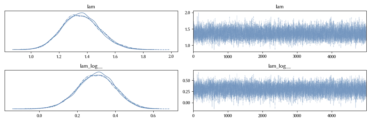
az.summary(trace_uncensored, var_names=['lam'])
| mean | sd | hdi_3% | hdi_97% | mcse_mean | mcse_sd | ess_bulk | ess_tail | r_hat | |
|---|---|---|---|---|---|---|---|---|---|
| lam | 1.358 | 0.135 | 1.108 | 1.613 | 0.001 | 0.001 | 9201 | 13739 | 1 |
From the above summary we can observe that the $94\%$ HDI for this model does not contain the true value for the parameter.
Naive method 2: dropping the unobserved units
Another wrong method to deal with censoring is to only include in our dataset units which has an observation, while excluding the remaining.
w_1 = w[w<c]

with pm.Model() as dropped_model:
    lam = pm.Exponential('lam', lam=0.5)
    y = pm.Exponential('y', lam=lam, observed=w_1)
    trace_dropped = pm.sample(**kwargs)

az.plot_trace(trace_dropped)
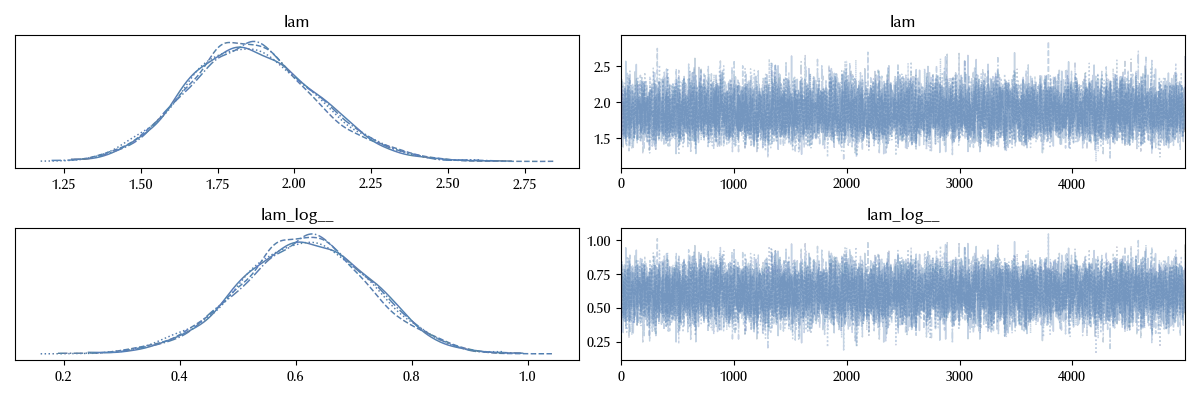
az.summary(trace_dropped, var_names=['lam'])
| mean | sd | hdi_3% | hdi_97% | mcse_mean | mcse_sd | ess_bulk | ess_tail | r_hat | |
|---|---|---|---|---|---|---|---|---|---|
| lam | 1.862 | 0.209 | 1.478 | 2.265 | 0.002 | 0.001 | 9478 | 14163 | 1 |
This estimate is even worse than the above one.
Correct method
Let us now show that a correct inclusion of the censoring into the model gives a better estimate of the average lifetime. In PyMC, censoring can be simply implemented by using the Censored class.
with pm.Model() as censored_model:
    lam = pm.Exponential('lam', lam=0.5)
    dist = pm.Exponential.dist(lam=lam)
    y_censored = pm.Censored('y_censored', dist, observed=w_cp, upper=c, lower=None)
    trace_censored = pm.sample(**kwargs)

az.plot_trace(trace_censored)
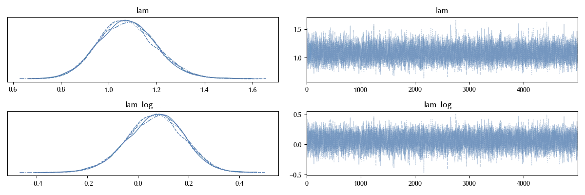
az.summary(trace_censored, var_names=['lam'])
| mean | sd | hdi_3% | hdi_97% | mcse_mean | mcse_sd | ess_bulk | ess_tail | r_hat | |
|---|---|---|---|---|---|---|---|---|---|
| lam | 1.078 | 0.12 | 0.859 | 1.307 | 0.001 | 0.001 | 8974 | 13740 | 1 |
We now have that our estimate is correct within one standard deviation, and this is a huge improvement with respect to both the naive methods.
Comparison of the results
In order to better understand the difference in the estimate, let us now sample and plot the posterior predictive distributions of the three models.
with censored_model:
    y_pred = pm.Exponential('y_pred', lam=lam)
    ppc_censored = pm.sample_posterior_predictive(trace_censored, var_names=['y_pred'])

with uncensored_model:
    y_pred = pm.Exponential('y_pred', lam=lam)
    ppc_uncensored = pm.sample_posterior_predictive(trace_uncensored, var_names=['y_pred'])

with dropped_model:
    y_pred = pm.Exponential('y_pred', lam=lam)
    ppc_dropped = pm.sample_posterior_predictive(trace_dropped, var_names=['y_pred'])
bins = np.arange(0, 10, 0.5)
xlim = [0, 10]
ylim = [0, 1.2]

xticks = [0, 5, 10]
yticks = [0, 0.5, 1]

fig = plt.figure(figsize=(12, 4))

ax1 = fig.add_subplot(131)
ax1.hist(ppc_uncensored.posterior_predictive['y_pred'].values.reshape(-1), density=True, bins=bins,  alpha=0.8)
ax1.hist(w, density=True, bins=bins, alpha=0.6)
ax1.set_title('Uncensored')
ax1.set_xlim(xlim)
ax1.set_ylim(ylim)
ax1.set_xticks(xticks)
ax1.set_yticks(yticks)

ax2 = fig.add_subplot(132)
ax2.hist(ppc_dropped.posterior_predictive['y_pred'].values.reshape(-1), density=True, bins=bins,  alpha=0.8)
ax2.hist(w, density=True, bins=bins, alpha=0.6)
ax2.set_title('Dropped')
ax2.set_xlim(xlim)
ax2.set_ylim(ylim)
ax2.set_xticks(xticks)
ax2.set_yticks(yticks)

ax3 = fig.add_subplot(133)
ax3.hist(ppc_censored.posterior_predictive['y_pred'].values.reshape(-1), density=True, bins=bins,  alpha=0.8)
ax3.hist(w, density=True, bins=bins, alpha=0.6)
ax3.set_title('Censored')
ax3.set_xlim(xlim)
ax3.set_ylim(ylim)
ax3.set_xticks(xticks)
ax3.set_yticks(yticks)

fig.tight_layout()
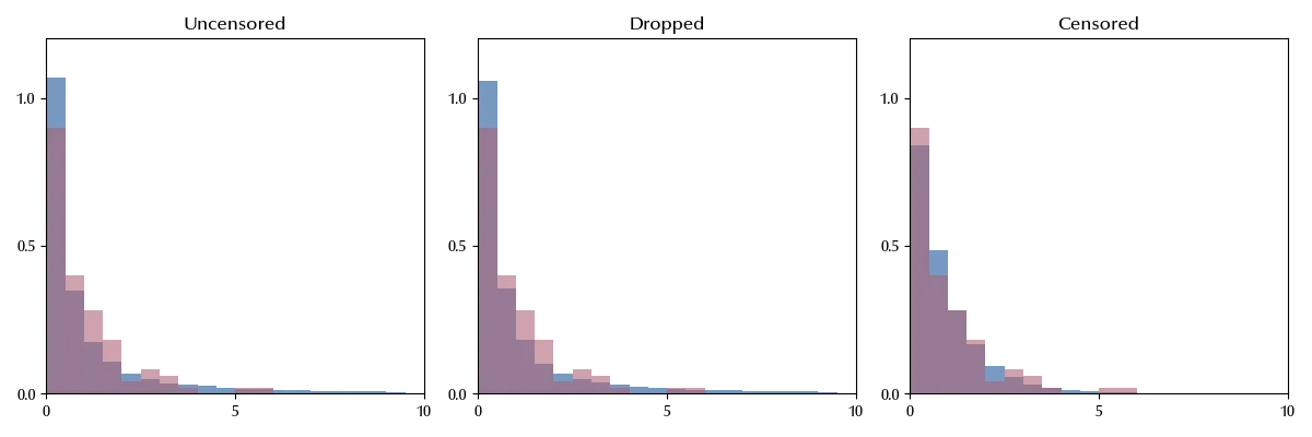
In the above figures, the red histogram corresponds to the true (uncensored) data, while the blue one corresponds to the posterior predictive distribution of our model. The effect of the bias for method 1 and 2 is quite evident, while the censored model predicts a distribution which is quite close to the true data.
Let us also compare the different estimates of the parameter
fig, ax = plt.subplots()
az.plot_forest([trace_uncensored, trace_dropped, trace_censored],
               var_names='lam', combined=True,
               model_names=['threshold', 'dropped', 'censored'], ax=ax)
ax.axvline(x=1, color='lightgray', ls='--')
ax.annotate('True value', (1.02, 3.3), color='gray', fontsize=15)
fig.tight_layout()
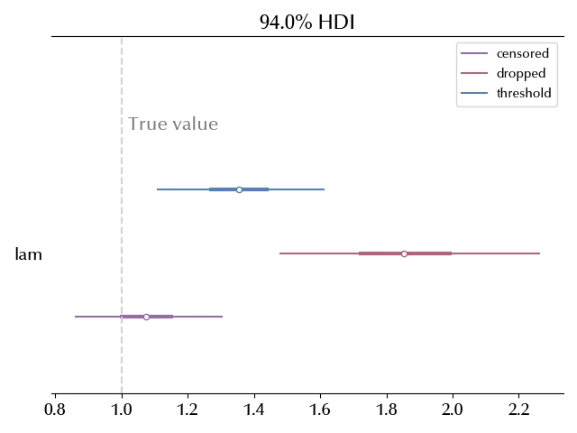
As you can see, the only reliable estimate is the censored one, while the remaining models are overestimating the true parameter value.
Conclusions
We introduced survival analysis, and we introduced some main concept as the hazard function and the survival function. We also discussed censorship, and we showed with an example why it is important to correctly account of censoring. You should keep in mind that there’s no way your model knows about censoring from the data, the only way to implement it is to build a model where it is implemented by you.
%load_ext watermark
%watermark -n -u -v -iv -w -p xarray,numpyro,jax,jaxlib
Python implementation: CPython
Python version : 3.13.9
IPython version : 9.7.0
pytensor: 2.35.1
xarray : 2025.1.2
numpyro : 0.19.0
jax : 0.8.0
jaxlib : 0.8.0
nutpie : 0.16.2
numpy : 2.3.4
arviz : 0.23.0.dev0
matplotlib: 3.10.7
pymc : 5.26.1
seaborn : 0.13.2
Watermark: 2.5.0